From: AAAI Technical Report FS-92-04. Copyright © 1992, AAAI (www.aaai.org). All rights reserved.
Context
Space
Hinrich Schfitze
Center for the Study of Languageand Information
VenturaHall
Stanford University
Stanford, California 94305-4115
schuetze@csli.stanford.edu
Abstract
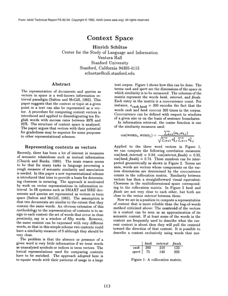
text corpus. Figure 1 shows how this can be done. The
terms cash and sport are the dimensions of the space in
which similarity is to be measured. The columnsof the
matrix represent the words bank, interest, and finals.
Each entry in the matrix is a cooccurrence count. For
instance, acash, bank = 300 encodes the fact that the
words cash and bank cooccur 300 times in the corpus.
Cooccurrence can be defined with respect to windows
of a given size or on the basis of sentence boundaries.
In information retrieval, the cosine function is one
of the similarity measures used:
Tile representation of documents and queries as
vectors in space is a well-known information retrieval paradigm (Salton and McGill, 1983). This
paper suggests that the context or topic at a given
point in a text can also be represented as a vector. A procedure for computing context vectors is
introduced and applied to disambiguating ten English words with success rates between 89% and
95%. The structure of context space is analyzed.
The paper argues that vectors with their potential
for gradedness maybe superior for some purposes
to other representational schemes.
Representing
contexts
COS(WORDi,
as vectors
Recently, there has been a lot of interest in measures
of semantic relatedness such as mutual information
(Church and Hanks, 1989). The main reason seems
to be that for many tasks in language processing a
rough measure of semantic similarity and association
is needed. In this paper a new representational scheme
is introduced that tries to provide a basis for determining closeness in meaning. The approach is motivated
by work oil vector representations in information retrieval. In IR systems such as SMART
and SIRE documents and queries are represented as vectors in term
space (Salton and McGill, 1983). The assumption
that two documents are similar to the extent that they
contain the same words. An obvious extension of this
methodologyto the representation of contexts is to assign to each context the set of wordsthat occur in close
proximity, say in a windowof fifty words. However,
the same content can be expressed with very different
words, so that in this simple schemetwo contexts could
have a similarity measure of 0 although they should be
very close.
The problem is that the absence or presence of a
given word is very little information if we treat words
as unanalyzed symbols or indices in term vectors. The
lexical representations used for comparing contexts
have to be enriched. The approach adopted here is
to equate words with their patterns of usage in a large
113
WORDj) =
~
~=l(ak’iak’J)
n a 2 X-,n
_2
k=l k,i /--~k=l t*k,j
Applied to the three word vectors in Figure 1,
we can compute the following correlation measures:
cos(bank, interest) = 0.94, cos(interest, finals) = 0.92,
cos(bank, finals) 0. 74. These numbers can be int erpreted geometrically as shown in Figure 2. Terms are
axes, words are vectors whose components on the various dimensions are determined by the cooccurrence
counts in the collocation matrix. Similarity between
vectors has then a straightforward visual equivalent:
Closeness in the multidimensional space corresponding to the collocation matrix. In Figure 2 bank and
finals are not very close to each other, but both are
close to the vector interest between them.
Nowwe are in a position to computea representation
of context that is more reliable than the bag-of-words
method criticized above: The centroid of the vectors
in a context can be seen as an approximation of its
semantic content. If at least some of the words in the
context are frequently used to describe what the current context is about then they will pull the centroid
toward the direction of that content. It is possible to
describe a content exclusively using words that nor-
cash
sport
J
bank
300
75
interest
210
140
finals
133
200
Figure 1: A collocation matrix.
From: AAAI Technical Report FS-92-04. Copyright © 1992, AAAI (www.aaai.org). All rights reserved.
cash
300
/
inlerest
ban/tex~
133
jn~nal
s
75
200
sporl
Figure 2: A vector model for context.
really express unrelated thoughts. But those contexts
are exceptions. -- In tile experiments described here, a
"saw tooth" weighting function is used for computing
tile context vector. It emphasizes words close to the
context over those that are distant.
Let us look at word sense disambiguation to see how
this representation of context can be put to work. Consider the example of interest. Let PERCENTbe the tag
for uses of interest in the sense "charge on borrowed
money" and CONCERN
the tag for "a feeling that accompanies or causes special attention." Then the PERCENT
sense will occur more often in contexts that score
high on the cash dimension. On the other hand, sport
will cooccur with the CONCERN
sense more often than
with the PERCENT
sense. Wecan then disambiguate
an occurrence of interest at a given position in the text
by computing the context vector of that position and
determining how close it is to the cash and sport dimensions of the space. Two such context vectors are
depicted in Figure 2. Vector contextl is closer to cash,
so probably it is an occurrence of the PERCENT
sense
of interest. Vector context2 is closer to sport, and it
will be an occurrence of the CONCERN
sense.
A space with only two dimensions, cash and sport,
would make for a rather impoverished representation.
For good results, several thousand words have to be
used. Since dense vectors in high-dimensional spaces
are computationally inefficient a space reduction by
means of a singular value decomposition is necessary,
along the lines of (Deerwester el al., 1990). See
(Sch/itze, 1992) for a more detailed description of how
to computethe initial vector representations for words.
114
Word sense
disambiguation
The main problem in using vector representations
for disambiguation is to find the directions in the
space that correspond best to the various senses of
an ambiguous word. One could imagine many labourintensive ways of identifying such directions: for instance finding several dozen typical uses and computing their centroid. A less reliable, but automatic
methodis to cluster a training set of contexts, to assign senses to the clusters and to assign to new occurrences the sense of the closest cluster. This approach
was taken here. The clustering programs used are AutoClass (Cheeseman el al., 1988) and Buckshot (Cutting el al., 1992). AutoClass is a Bayesian classification program based on the theory of finite mixtures.
It determines the number of clusters automatically by
imposing a penalty on each new cluster and thus counterbalancing the fact that moreclusters will necessarily
better account for the data. Due to the computational
complexity of high-quality classification, a more efficient, linear algorithm was used for some of the large
data sets shown in Table 1. Buckshot clusters n items
by applying a quadratic high-quality clustering algorithm to a random sample of size x/~ and extending
this classification in linear time to the rest of the data
set.
Table 1 summarizes the ten disambiguation experiments that have been conducted so far. The first columncontains the word that is to be disambiguated. In
two cases, inflected forms are excluded because they
are not ambiguous. (rulings only has the decision
sense, spaces cannot mean "outer space.") For all
words, training and test set were taken from the New
York Times NewsService 1989 and 1990. 9 and 0 to the
From: AAAI Technical Report FS-92-04. Copyright © 1992, AAAI (www.aaai.org). All rights reserved.
word
training set
test set
# contexts per sense
%correct
09
tank/s
planl/s
interest/s
capital/s
suit/s
motion/s
ruling
vessel/Is
space
train/s
0:6-0:10
1780
0:6-0:10
4132
0:6-0:7
2955
0:6-0:8
2000
9:5-0:10
8206
9:5-0:10
3101
9:5-0:10
5966
9:6-0:10
1701
9:5-0:10 10126
9:5-0:10 4775
months
0:11
0:11
0:11
0:11
0:11
0:11
0:11
9:5,0:11
0:11
0:11
% -~
336 A
502 A
501 A
200 A
498 B
200 B
200 B
144 B
200 B
266
8
13
3
2
2
2
2
7
10
16
14
15
5
18
0
4
10
0
8O
66
68
66
54
54
6O
58
59
1
2
226 56
283 188
291 165
127 64
220 189
107 93
115 78
76
23
118 82
200
62
3
22
sum
1
282 97
471
94
456 94
191 96
409 94
200 92
193 90
130
93
200 89
262 94
Table 1: Ten disambiguation experiments.
word
~ank//s
plant/s
interest/s
capital/s
suit/s
motion/s
ruling
vessel/s
space
train/s
1
2
1
2
1
2
1
2
1
2
1
2
1
2
1
2
3
N
N
N
NV
NV
N
N
N
N
N
N,
N
NV
V
N
N
N
definition
heavily armed combat vehicle
receptacle for holding liquids
a factory for the manufacture of a particular product
living beings typically lacking locomotive movement
a feeling that accompaniesor causes special attention
a charge for borrowed money
a stock of accumulated goods
a city serving as a seat of government
an action or process in a court
a set of garments
movement
a proposal for action
an official or authoritative decision
to exert control, direction, or influence
a hollow structure designed for navigation
blood vessel
a hollow or concave utensil
extent in one, two, or three dimensions
the region beyond the earth’s atmosphere
a connected line of railroad cars
to teach so as to makefit, qualified, or proficient
Table 2: Definition of the senses in Table 1.
115
2
3 sum
85
95
88
92
92
93
92
95
95
95
91
92
91
90
91 86
92
90
90
69
89
From: AAAI Technical Report FS-92-04. Copyright © 1992, AAAI (www.aaai.org). All rights reserved.
left of the colon abbreviate 1989 and 1990, the number
after tile colon encodes tile month. For example, vessel was trained on all months between June 1989 and
October 1990 and tested on May 1989 and November
1990. Columns 3 and 5 show how often the ambiguous word occurred in test and training set. Column6
has "A" for AutoClass and "B" for Buckshot. Column
7 gives the number of classes found by AutoClass or
the numberof classes requested for Buckshot. Usually,
classifications with 2, 5, 7 and 10 classes were tried.
The first successful trial is reported in the table.
Infrequent senses of the ambiguous words were excluded here. The percentage in column 8 indicates how
many occurrences are not accounted for. It also includes repetitions of identical contexts for tank, plant,
interest, suit, and vessel. For these words repeated
contexts only count once.
The column "major sense" shows how dominant the
major sense of the word is. For instance, 80%of the
frequent uses of tank are "vehicle" uses, 20%"receptacle" uses.
The last six columnsof the table contain the absolute
number of occurrences per sense and the percentages
of correct disambiguation.
It is important to note that senses were assigned to
classes on the basis of the training set. In the case
of autoclass, only classes that had at most two errors
amongthe first 10 memberswere assigned. In the case
of buckshot, the majority of the first 10 or 20 members
determined sense assignment. It is always possible to
combineclasses in the test set to get good results. In
the extreme case, a classification with as manyclasses
as items in the data set is guaranteed to be 100%correct. But since classes were assigned using the training
set here, even a high number of classes seems unproblematic.
Table 2 glosses the major senses of the ten words.
Somesenses can be realized as verbs or nouns. In general, verbs are harder to disambiguate than nouns, but
as tile results for plant, interest, ruling and train show,
success ill the 90070range is possible.
The senses that occurred ill the NewYork Times
and were excluded are "tank top" and "think tank"
for tank; metaphorical senses such as "to plant a suction cup Garfield" for plant; the "legal share" sense
of interest; the adjectival and sports senses of capital
("capital punishment", "Washington Capitals"); the
verbal sense of suit ("to be proper for"), the card game
sense and "to follow suit"; "to rule out" for ruling; and
"an orderly succession" and "drive-train" for train.
Analyzing
context
space
Howcan the results in Table 1 be improved? There
are many parameters that had to be fixed rather arbitrarily and they may have gotten suboptimal settings.
This section investigates three of them: the size of the
window;the weighting of the dimensions of the space;
and the selection of different sets of dimensions.
116
Window
Size
In Table 1, a windowof 1200 characters was used for
tank and plant and a window of 1000 characters for
the other words. It makes more sense to limit the window by the number of characters than by the number
of words because few long words are as good as (or
even better) than many short words which tend to be
high-frequency and function words. Howdoes window
size influence disambiguation performance? To answer
this question one could cluster context sets that are
computed with varying windowsizes. However, there’s
some variability in the results of clustering and the
best window size may yield mediocre disambiguation
results by accident. A deterministic method is therefore needed.
Canonical Discriminant Analysis (CDA) or linear
discrimination is such a method (Gnanadesikan, 1977).
It finds the best weighting or linear combination of the
dimensions of the space so that the ratio of the sum
of between-group distances to the sum of the withingroup distances is maximized.This task is slightly different from classification. It could be that, say, fourty
dimensions are sufficient for clustering, but that you
need more to tease the two words apart on a linear
scale as CDAdoes. Conversely, even though giving
large weights to few dimensions with very low values
in the original space can result in a nice separation, a
clustering procedure may not be able to take advantage of this situation because the distance measure is
the cosine and it concentrates on dimensions with high
values. So the results below have to be interpreted
with some caution.
Linear discrimination
is a supervised learning
method: The items in the training set have to be
labelled. Since labelling thousands of instance of
ambiguous words is not feasible, a simple trick was
employed here. Instead of discriminating
an ambiguous word for which the sense tags in the corpus are unknown, three artificial
ambiguous words
were created: author~baby, giants~politicians,
and
train~tennis. These pairs were selected because the
words in each pair are comparable in frequency in the
corpus; and they are as distinct semantically as the different senses of ambiguouswords like suit or capital.
All six words are nouns because the meaning of verbs
often depends on their arguments rather than on the
general context. However, about twenty percent of the
occurrences of train are verbal (see above). Table
lists the frequencies of the CDAwords in training and
test set.
Figure 3 shows how generalization to the test set
depends on the number of dimensions and the window
size. The solid line is 1200 characters, the dense dotted line 1000 characters and the sparse dotted line 800
characters. Each point in the graph was computed as
follows: For a given windowsize, a linear discrimination analysis was performed for the 3096 data points in
the training set using the first n dimensions, where the
From: AAAI Technical Report FS-92-04. Copyright © 1992, AAAI (www.aaai.org). All rights reserved.
90%
.......
°°°.o~....
.. I ¢ :. ..............
.....Oo....
°_,~*° °. °..
80%
I
40
3O
I
50
I
60
I
70
a
80
f
90
70%
Figure 3: Three windowsizes for discriminating author/baby.
pair
word
pair 1 author
baby
pair 2 train
tennis
pair 3 giants
politicians
frequency in
training set test set
Jun90-Oct90
Nov90
1552
312
1544
349
1089
219
1072
136
1544
707
1530
364
Table 3: Frequency of tile
flattens out fast beyond dimension 96. The discrimination graph for giants/policiticans has a very clear
rising tendency, so an improvementin perfomance with
more dimensions seems likely.
Dimension
words used in CDA.
value of n is indicated on the horizontal axis. The computed weighting was used to project the 3096 points
onto one dimension. The optimal cutting point was determined. The projection and the cutting point were
then applied to the test set. The graph shows how
manycontexts in the test set were discriminated correctly.
Apparently, 1000 characters is the ideal window
size for discriminating author/baby. The results for
train~tennis were similar in that 1000 characters
seemed the optimal size most of the time although 1000
and 1200 characters produced almost identical generalization for manydimensions. For giants~politicians,
the graphs for tile three windowsizes were almost identical for most dimensions. This suggests that 1000
characters is a good window size for computing the
context vector.
Figure 3 also suggests that using more than 97 dimensions would improve the disambiguation results.
Unfortunately, only 97 dimensions were extracted
when computing the singular value decomposition, so
it couldn’t be tested whether the curve keeps rising or
117
weights
The second question is whether all dimensions are important for some distinctions or whether there are some
that are never used. A preliminary answer can be
found in Figures 5 and 6. They show the optimal
weights as computed by the CDAalgorithm if all 97
dimensions are used. Dimensions 0,10, 20, 30, 40, 50,
60, 70, 80, and 90 are markedon the horizontal axis in
both figures. The height of each rectangle shows the
relative weight of the corresponding dimension. The
weightings were very stable when new dimensions were
added, with each incoming dimension dampening the
weights of the others without changing the "gestalt" of
the weight graph.
Different weightings seem to be necessary for different word pairs. For instance, dimension 10 (the second
markeddimension from the left) has weigth zero for author~baby, but a high positive weight for train~tennis.
Dimensions 70 and 80 (the second and third marked
dimensions fro mthe right) have weights with the same
signs for author~baby and weights with different signs
for train~tennis. So whereas high positive values on
both 70 and 80 will strongly favor one sense over the
other in discriminating author~baby, they cancel each
other out for train~tennis. The optimal weights for
giants/politicians
display yet another pattern. This
evidence suggests that different dimensions are important for different semantic distinctions and that all are
potentially useful.
From: AAAI Technical Report FS-92-04. Copyright © 1992, AAAI (www.aaai.org). All rights reserved.
90%
8O%
I
80
I
70
I
60
I
50
I
40
I
30
I
20
I
10
I 70%
0
Figure 4: Generalization for final dimensions in discriminating author/baby.
Figure 5: Optimal dimension weights for discriminating author/baby.
’u u ~’ ,,~ ’~kl’uo
I
ll}U"
Figure 6: Optimal dimension weights for discriminating train/tennis.
118
[_
7
From: AAAI Technical Report FS-92-04. Copyright © 1992, AAAI (www.aaai.org). All rights reserved.
Selection
of dimensions
Three experiments were conducted to find out whether
some groups of dimensions were more important than
others. In general, a singular value decomposition
yields a space in which the first dimension is most
important, the second dimension is the second most
important etc. But this doesn’t seem to be the case
here as the disambiguation results in Table 4 and Figure 4 show. Data set 1 (contexts of suit) in Table 4
was first classified using only dimensions 1 through 30.
The error rate on the test set was 6%. Then a classification with the last 38 dimensions was computed,
yielding an error rate of 6%. Finally, all 97 dimensions
except for the very first one were classified. Here, the
error rate was 5%. This suggests that the vector representations are highly redundant and that the result
of tile singular value decomposition computed here is
different from other SVDapplications in that the first
one hundred dimensions are all equally meaningful for
tile disambiguation task. This hypothesis is confirmed
by the classification of the second data set in Table 4.
Using all 30 dimensions, tile error rate is 9%. Deleting
either all even dimensions or all odd dimensions causes
an increase of the error rate, but there’s still enough
information to find a classification of moderatequality.
data set 1
data set 2
dimensions used
1-30
59-96
1-96
1,2,3,...,29,30
1,3,5,...,27,29
2,4,6,... ,28,30
performance measured in percent correct/percent incorrect. However, no clear distinction between training set and test set is made. The assignment of Roget’s
categories to the different senses of an ambiguousword
is apparently done by hand. It is not clear how well
the heuristics used for this process wouldextend to unseen data, especially for senses that occur only once in
Grolier’s. Yarowsky’s method is clearly superior when
it comes to identifying senses with a frequency of less
than twenty percent. But there are many domains and
languages without thesauri and tagger, so that it isn’t
as broadly applicable as the algorithm introduced here.
In another recent paper, Gale et al. claim that
there’s an upper bound on the level of performance
for word sense disambiguation due to the inability of
human judges to agree on sense tag assignment. An
example for a context that humanjudges will differ
on could be the following sentence from the NewYork
Times:
In Texas, Williams, a millionaire businessman
with interests in oil, cattle and banking, was hurt
among voters who considered ethics an important
issue.
This sentence maybe assigned to "legal share" as well
as % feeling that accompanies special attention." In
fact, it should be assigned to both senses at the same
time, since both senses seem to be activated in the
context. If exampleslike these are typical, conflicting
sense assignments could be an artifact of the sense disambiguation’task. The assumption is that there’s one
sense tag to assign, cases of polysemyor intermediate
meaning are not taken into consideration. What this
calls for is a framework that allows for intermediate
sense tags. The vector space introduced here seems to
provide a good starting point for dealing with polysemy. A given context need not be categorized using
a limited set of tags. Instead, its distance from previous contexts and arbitrary lexical items can be computed - fairly reliably as the disambiguation results
presented here suggest. For many tasks in computational linguistics such as PP attachment or machine
translation, such a flexible tool could be more useful
than the Procrustean bed of predefined tags.
error rate
6%
6%
5%
9%
14%
13%
Table 4: Sublexical representations are distributed.
Finally, Figure 4 is evidence that the very first dimensions may actually have less relevant information
in them than the immediately following ones. Figure 4
was computed in analogy to Figure 3, but here sets
of final dimensions were used for CDA(instead of sets
of initial dimensions). So the data point at position
80 shows the generalization on the test set when dimensions 80-96 are used etc. Disambiguation on the
basis of the last fourty dimensions attains ahnost optimal performance and adding dimensions 0-50 only
leads to minor improvements. The curve is initially
nmch steeper than its counterpart in Figure 3. Further research is necessary to find out whether dimensions 100-200 are even better than 50-100. In any case,
some hope seems justified that disambiguation in context space can be improved.
Acknowledgements
I’m indebted to John Tukey for suggesting the use of
CDA,and to Martin Kay and Jan Pedersen for discussions and help.
I’m grateful to Mike Berry for SVDPACK;
to NASA
and RIACSfor AutoClass; to the San Diego Supercomputer Center for providing seed time; and to Xerox
PARCfor making corpora and corpus tools available
to me.
Discussion
In a recent paper, David Yarowsky presents a disambiguation model based on Roget’s thesaurus (1992).
His method seems slightly more successful in terms of
References
Berry, Michael Waitsel 1992. Large scale singular
119
From: AAAI Technical Report FS-92-04. Copyright © 1992, AAAI (www.aaai.org). All rights reserved.
value computations. Int. J. of Supercomputer Applications 6(1): 13-49.
Cheeseman, Peter; Kelly, James; Self, Matthew;
Stutz, John; Taylor, Will; and Freeman, Don 1988.
Autoclass: A bayesian classification system. In Proceedings of the Fifth International Conference on Machine Learning, Ann Arbor: University of Michigan.
Church, Kenneth Ward and Hanks, Patrick 1989.
Wordassociation norms, mutual information and lexicography. In Proceedings of the 27th Annual Meeting
of the Association for Computational Linguistics.
Cutting, Doug; Karger, David; Pedersen, Jan; and
Tukey, John 1992. Scatter-gather:
A cluster-based
approach to browsing large document collections. In
SIGIR ’92 Copenhagen.
Deerwester, Scott; Dumais, Susan T.; Furnas,
George W.; K.Landauer, Thomas; and Harshman,
Richard 1990. Indexing by latent semantic analysis.
Journal of the American Society for Information Science 41(6):391-407.
Gale, William;
Church, Kenneth Ward; and
Yarowsky, David 1992. Estimating upper and lower
bounds on the performance of word-sense disambiguation programs. In Proceedings of the 30th Annual
Meeting of the Association for Computational Linguistics.
Gnanadesikan, 1977. Methods for Statistical
Data
Analysis of Multivariate Observations. John Wiley
& Sons, NewYork.
Salton, Gerard and McGilI, Michael J. 1983. b~troduction to modern information retrieval. McGraw-Hill,
New York.
Schiitze, Hinrich 1992. Wordsense disambiguation
with sublexical representations.
In AAAI Workshop
Notes: Statistically-Based NLPTechniques. San Jose.
Yarowsky, David 1992. Word-sense disambiguation
using statistical modelsof roget’s categories trained
on large corpora. In Coling 92.
120