Integration of Probabilistic Graphic Models for Decision Support
Chang-an JIANG, Kim-leng POH, Tze-yun LEONG
National University of Singapore
Medical Computing Lab, School of Computing, NUS, 117543, Singapore
Department of Industrial and Systems Engineering, NUS,119260, Singapore
{ChanganJiang, isepohkl}@nus.edu.sg leongty@comp.nus.edu.sg
Abstract
Operation
Skin Damification
It is a frequently encountered problem that new knowledge
arrived when making decisions in a dynamic world. Usually,
domain experts cannot afford enough time and knowledge to
effectively assess and combine both qualitative and quantitative information in these models. Existing approaches can
solve only one of two tasks instead of both. We propose a
four-step algorithm to integrate multiple probabilistic graphic
models, which can effectively update existing models with
newly acquired models. In this algorithm, the qualitative part
of model integration is performed first, followed by the quantitative combination. We illustrate our method with an example of combining three models. We also identify the factors
that may influence the complexity of the integrated model.
Accordingly, we identify three factors that may influence the
complexity of the integrated model. Accordingly, we present
three heuristic methods of target variable ordering generation.
Such methods show their feasibility through our experiments
and are good in different situations. Finally, we provide some
comments based on our experiments results.
Inflammation
Fever
Permanent Scar
Death
(a) From dermatology literature
Operation
Operation
Skin
Damification
Fever
Vein
Damification
Thrombus
Nerve
Damification
Bleeding
Paralysis
Nerve Damification
Coma
Paralysis
Kidney
Syndrome
Lung
Syndrome
Death
Death
(b) From surgery domain expert
(c) From surgery
domain expert
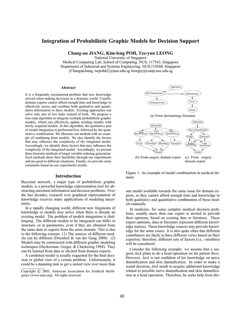
Figure 1: An example of model combination in medical domain
Introduction
Bayesian network, a major type of probabilistic graphic
models, is a powerful knowledge representation tool for abstracting uncertain information and decision problems. Over
the last decades, research over graphical representation of
knowledge receives many applications of modeling uncertainty.
In a rapidly changing world, different new fragments of
knowledge or models may arrive when there is already an
existing model. The problem of models integration is challenging. The different models to be integrated can differ in
structure, or in parameters, even if they are obtained from
the same data or experts from the same domain. This is due
to the following reasons: (1) The sources of different models can be different (Druzdzel & van der Gaag 2000). (2)
Models may be constructed with different graphic modeling
techniques (Heckerman, Geiger, & Chickering 1994). They
can be learned from data or elicited from domain experts.
A combined model is usually requested for the final decision or global view of a certain problem. Unfortunately, it
could be a daunting task to get a united view over more than
one model available towards the same issue for domain experts, as they cannot afford enough time and knowledge to
both qualitative and quantitative combination of these models manually.
In medicine, for some complex medical decision problems, usually more than one expert is invited to provide
their opinions, based on existing data or literature. These
expert opinions, data or literature represent different knowledge sources. These knowledge sources may provide knowledge for the same issues. It is also quite often that different
contributors are likely to have different views based on their
expertise; therefore, different sets of factors (i.e., variables)
will be considered.
Consider the following example: we assume that a surgeon Jack plans to do a head operation on his patient Rose.
However, Jack is not confident of his knowledge on nerve
damnification and skin damnification. In order to make a
sound decision, Jack needs to acquire additional knowledge
related to possible nerve damnification and skin damnification in a head operation. Therefore, he seeks help from der-
c 2005, American Association for Artificial IntelliCopyright gence (www.aaai.org). All rights reserved.
40
matology literature and neurology data set.
This example case on a forthcoming head operation is
shown in Figure 1. Three Bayesian networks are modeled
from dermatology literature, a surgeon’s domain expertise
(i.e., Jack) and neurology data set respectively. The variables operation and death exist in all of the three networks.
The first network and the second network have another two
common variables—skin damnification and fever. The second network and the third network contain another two
common variables—nerve damnification and paralysis. Although there are some common variables between any two
networks, the structures are different. For example, there is
a direct arc from skin damnification to fever in the second
network, while there is no direct arc in the first network. In
the second network, there is no link from variable paralysis
to variable death, while there is a route from paralysis to
death through lung syndrome. This example is a simplified
version of real medical problems. In fact, real medical problems usually involve a large number of variables, complex
relationships among the variables, and numerous parameters.
Some research (Clemen & Winkler 1999; Maynard-Reid
& Chajewska 2001) has been done on combining probability
distributions. Some merely address topology combination in
BNs (Matzkevich & Abramson 1992; Joseph, Parmigiani, &
Hasselblad 1998), which only two models can be combined
at one time. Besides of shortcoming of unscalability, the
resulting model can also influenced by the order of combination, if there are more than two models to be combined.
In this paper, we present an approach to solve both
of qualitative and quantitative combination of an arbitrary
number of probabilistic graphical models at a time. Our approach also provides a natural way and simple base for CPT
combination.
Furthermore, we present three heuristic methods for automatic generation of target variable ordering for the resulting
model.
We make two intuitively reasonable assumptions for
model combination: (1) Variables with same name model
the same real world entity. (2) Variables with same name
have to be over the same domains (in the discrete case, the
same set of possible states).
E
A
B
B
M
N
A
B
F
C
D
(a) Candidate BN 1 (b) Candidate BN 2 (c) Candidate BN 3
Figure 2: Example of three candidate Bayesian networks
dependency among variables; and the quantitative part that
numerically represents the joint probability distribution over
these variables.
There are four major challenges in this task. The first
challenge lies in the qualitative combination: how to avoid
cycles after combination of multiple Bayesian networks. Direct combination of different models can result in cycle(s) in
the resulting model. Figure 3 presents two examples of possible situations in DAG (Directed Acyclic Graph) that may
incur a cycle in combination. We name these two situations
as direct conflict cases and indirect conflict cases. The problem of avoiding a possible cycle can be solved using the
arc reversal operation (Shachter 1984), which was applied
in topology combination (Matzkevich & Abramson 1992) .
A
A
A
B
B
B
(a)
(b)
(c)
(a) Direct conflict
A
A
A
B
D
B
D
C
C
(a)
C
(b)
(c)
(b) Indirect conflict
Problem Formulation and Challenges
We assume a finite number of Bayesian networks B1 , .., Bm .
−
→
→
−
Bi = (Vi, Ei ) where i = 1, 2, ...m, and E = (a, b) denote
directed edges between every pair of nodes a and b within
one probabilistic graphic model. The direction of edge is
from a to b, which we denote < a, b >. These m Bayesian
Tm −
Tm
→
networks can satisfy φ ⊆ i=1 Vi and φ ⊆ i=1 Ei .
These available probabilistic graphic models to be combined are termed as candidate Bayesian networks. To combine the Bayesian networks, we aim at getting a single BN
Sm −
→
model. In general Eresult = i=1 Ei is true only in some
special cases. An example of three different Bayesian networks is shown in Figure 2.
Each Bayesian network consists of two parts. The qualitative part that represents the structure of the network and
Figure 3: Conflict in DAG combination
The second challenge lies in the change of conditional independence relationships after combination. Adding an arc,
it will break some independent relationships among variables. In other words, we may focus on minimize additional dependence relationships between nodes in the resulting Bayesian network. Set operation over conditional independence statements was used (Sagrado & Moral 2003)
to solve the graph combination problem. Unfortunately, it
is not easy to perform parameter combination based on this
method.
41
G1
2. Adjust variable ordering and edge direction
G2
3. Save amended models as Intermediate Bayesian networks
M1
Gresult M 2
CI1
CIresult CI2
4. Combine CPT
Step 1: Re-organize Bayesian networks
According to the chain rule factorization property of BN,
a JPD (Joint Probability Distribution) can be factorized in
more than one way. Each factorization indicates a different
ordering of variables. When we change the ordering, we
actually are changing the factorization of JPD. Therefore,
we can always re-organize BN according to different partial
ordering of variables, while maintaining the same JPD.
Figure 4: Probabilistic graphic models combination
Figure 4 shows an example case of combination of two
probabilistic graphic models. M1 and M2 are the two candidate models to be combined. G1 and G2 are graphs that
correspond to M1 and M2 respectively. As M1 implies G1 ,
and G1 encodes the conditional independence CI1 in M1 ,
M1 is not only a valid probabilistic graphic model, but also
a perfect map of the underlying dependency. Therefore, the
problem that we are facing is to get the resulting Gresult
where the underlying CIresult breaks the least conditional
independency from CI1 and CI2 .
The third challenge concerns the quantitative computation. Different candidate Bayesian networks may have different structure, which means that the internal CPT (Conditional Probability Tables)s may be very different; not only in
numbers, but also in the size of CPT. For example, the value
of P (A) in Model 1 is different from the value of P (A) in
Model 2. The CPT over node B in Model 1 is not only different from the CPT over node B of Model 2 in numbers,
but also in CPT size, as shown in Figure 4. There is not a
good way of combining CPTs in models yet.
A
B
A
a1
a2
P(A)
0.7
0.3
B\A
b1
b2
a1
0.4
0.6
A
a2
0.1
0.2
D
B
(a) Model 1
A
a1
a2
P(A)
0.1
0.9
A
B\D
b1
b2
d1
0.15
0.85
D
d1
d2
d3
a1
d2
0.3
0.7
Step2: Adjust variable ordering to maintain DAG
Defn 1. Order Value. Given a DAG D = (V, E), the
Odervalue(v) of a node v ∈ V in DAG D is defined as
the longest path from a rooted node to node v.
Defn 2. Variable Ordering.
λ is the sequence of
Ordervalue(v) for all node v ∈ V in DAG D.
Defn 3. Target Variable Ordering. λresult is the final variable ordering of the combined Bayesian network.
Note that λresult will not necessarily be the same as that
of any candidate models, although it is possible.
Lemma Cycle can be avoided when every arc in the candidate Bayesian networks are from nodes with lower order
value to nodes with higher order value.
P(D)
0.2
0.2
0.6
d3
0.9
0.1
d1
0.11
0.89
a1
d2
0.1
0.9
Proof:
Given k Bayesian networks B1,..., Bk , λ1,..., λk are variable ordering in B1,..., Bk .
We assume there exists one arc ¡s1, s2 > in Bi , Bi ∈
{B1 , ..., Bk }, in which
d3
0.5
0.5
(b) Model 2
ordervalue(s1 ) ≥ ordervalue(s2 )
Figure 5: CPT disagreement in two models
(1)
is satisfied.
According to the definition of ordervalue in Bayesian networks, ¡s1, s2 > denotes an arc starts from s1 , and ends at
s2 . Therefore we can get
The fourth challenge in model integration is how to integrate more than two models at the same time. In some large
Bayesian network model learning problems, knowledge engineering sometimes learn some small part of Bayesian networks and then combine them into a global Bayesian network. We can imagine a possible case that there are many
small Bayesian networks to be combined. If all these models
can be combined at a time, some manual work or time can
be saved. Unfortunately, existing methods can only combine
two models at a time. This is also a problem that we attempt
to solve.
ordervalue(s2 )
ordervalue(s2 )
= max{ordervalue(P a(S1 ))}+1(2)
> ordervalue(s1 )
(3)
which is conflict with 1. Therefore, every arc in Bayesian
networks is from nodes with lower ordervalue to nodes with
higher ordervalue.
Arc Reversal to Adjust Variable Ordering. Arc reversal
is needed here so that variable ordering in these networks are
consistent with target variable ordering with preservation of
JPD, but with some structural changes (Howard & E 1981;
Olmsted 1983). The three candidate Bayesian networks after arc reversal can been seen in Figure 6.
Bayesian Networks Combination
The proposed algorithm for integration of multiple Bayesian
networks consists of four steps, as follows.
1. Reorganize original BN
42
CBN1
Node
Ordervalue(A)
Ordervalue(B)
1
Ordervalue(C)
2
CBN3
User Specified Target Ordering
1
1
1
0
2
2
A
B
6
0
Ordervalue(F)
Ordervalue(M)
0
7
Ordervalue(N)
0
8
F
N
C
D
F
(a) Intermediate BN1
5
A
B
M
D
4
0
E
E
N
M
3
1
Ordervalue(D)
Ordervalue(E)
CBN2
C
(b) Intermediate BN2
N
M
E
B
A
C
Table 1: Order values in candidate BNs and target ordering
D
F
(c) Intermediate BN3
E
A
B
B
M
N
A
B
Figure 7: Example of virtual nodes
F
C
D
M
(a) Reconstruct (b) Reconstruct Can- (c) Reconstruct CanCandidate BN1 didate BN2
didate BN3
A
E
B
N
Figure 6: Arc reversal results over three candidate BNs
D
C
D
F
F
(a) Intermediate BN1
Step 3: Intermediate Bayesian Networks
We present a new concept of Intermediate Bayesian Networks in the procedure of combination.
A
B
E
M
C
N
(b) Intermediate BN2
M
N
A
B
E
Defn 4. Intermediate Bayesian Networks. Given k candidate Bayesian networks to be combined, B1 , · · · , Bk . We
make an identical copy from both qualitative part and quantitative part of these candidate Bayesian networks and save
them as Intermediate Bayesian networks.
D
F
C
(c) Intermediate BN3
Figure 8: Example of virtual arcs
The advantages of intermediate BN include 1) The structure and parameters of original input BN models can remain
unchanged. 2) With intermediate BN, we may turn the two
tasks of qualitative combination and quantitative combination into the single task of CPT combination among a set of
intermediate BNs with isomorphic topology.
Virtual Nodes and Virtual Arcs. In order to get homogeneous structure for every intermediate BN, we present the
concept of virtual nodes and virtual arcs. Figure 7 shows the
example of virtual nodes.
Three Heuristic Methods of Target
VariableOrdering Generation
We notice that there are some factors, which will influence
the generation of target variable ordering: (1) Original order values of each variable; (2) Number of parents of each
variable; (3) Size of each candidate Bayesian Networks. According to the above factors, we present three heuristic methods for target variable ordering generation.
Step 4: CPT Combination
With the help of virtual nodes and virtual arcs, for candidate BNs to be combined, we can get intermediate BNs with
same topology. An example is shown in Figure 7. In the
CPT combination part, we suggest there are two solutions:
(1) Using weighted combination, we can get standard CPT
filled with point probability distributions in result BN. (2)
Using interval combination, we can get Interval Bayesian
Networks (Ha & Haddawy 1996).
Method 1: Target Ordering based on Original
Order Valules
The following algorithm describes a method of automated
target variable ordering generation–Order value based Target Variable Ordering Generation method. We also provide
the proof of the correctness of this method.
43
Algorithm 2 Target Variable Ordering Generation based on
Number of Parents and Network Size
Require: B1 , . . . , Bk , k ≥ 2 and Bi = (V, E), i = 1 . . . k
1: for i = 1 to k do
2:
∀v in Bi ,
Store N umP arentsi (v);
Store N etSizei (v); {N etSizei (v) denotes the size
of network that node v is in};
tempV aluei [v]=
N umP arentsi (N odeN um)∗N etSizei (N odeN um);
3: end for
4: Vresult = ∪ki=1 Vi {push all nodes from candidate BNs
into Vresult };
5: N odesN um = —Vresult —;
6: initiate an array
7: AllN odes[N odeN um]=
[N odeID, OrderV alue, N ewOrderV alue];
8: for i = 1 to N odeN um do
9:
T argetOrder[N odeN um]=
P
tempV aluei [N odeN um];
10: end for
11: sort
N odeN um
according
to
T argetOrder[N odeN um]and nodeID {for two
nodes with same TargetOrder[NodeNum], sort according to nodeID }
12: Assign N ewOrdervalue to each Node according to the
position of each node after sorting
Algorithm 1 Order value based Target Variable Ordering
Generation in BNs Combination
Require: B1 , . . . , Bk , k ≥ 2 and Bi = (V, E), i = 1 . . . k
1: for i = 1 to k do
2:
∀v in Bi , Store OrderV alue(v);
3: end for
4: Vresult = ∪ki=1 Vi {push all nodes from candidate BNs
into Vresult };
5: N odesN um = —Vresult —;
6: initiate an array
7: AllN odes[N odeN um]=
[N odeID, OrderV alue, N ewOrderV alue];
8: for i = 1 to N odeN um do
9:
for j = 1 to k do
10:
v=AllNode(NumNode);
Pk
11:
Sumv = j=1 OrderV alue(vk ) ;{sum the node’s
ordervalue in all candidate BNs}
NodeAppear[NodeNum]++;{count how many
models that this node exist}
12:
end for
13: end for
14: for i = 1 to N odeN um do
Sumv
;
15:
AverageOrder[N odeN um] = N odeAppear
16: end for
17: sort
AverageOrder[N odeN um] according to
averagedordervalue and nodeID {for two nodes
with same average ordervalue, sort according to nodeID
}
18: Assign N ewOrdervalue to each Node after sorting
Node
CBN 1
Num Parent(A)
Node
CBN1
Ordervalue(A)
Ordervalue(B)
Ordervalue(C)
1
Ordervalue(F)
CBN3
Average
Target Order
1
1
1
2*
0
2
2
3
1
2
2
1
1
Ordervalue(D)
Ordervalue(E)
CBN2
0
0
Num Parent(B)
1
Num Parent(C)
2
2*
0
0
0
0
0
Ordervalue(N)
0
0
0
TargetOrder
8
2*
0
2
11
3
0
6
1
8
2*
0
0
0
0
Num Parent(M)
0
0
0
Num Parent(N)
0
0
0
Num of Nodes
Ordervalue(M)
W eighteSum
1
0
Num Parent(F)
3
CBN 3
1
2
Num Parent(D)
Num Parent(E)
CBN 2
3
4
4
Table 3: Example of target ordering based on num of parents
and network size
Table 2: Example of target ordering based on original order
value
Method 3: Target Ordering based on Edge Matrix
In this method, we consider the relative difference in order value between every pair of nodes in the candidate
Bayesian networks. We construct the edge matrix, by storing
the difference in order value for each variable in candidate
Bayesian networks. Thus there are k edge matrix if there are
k candidate Bayesian networks. To get the target variable
ordering, we need to get a final edge matrix after computation over these k candidate Bayesian networks. According
to the final edge matrix, we may get the relative difference
in order value of between each pair of nodes in the resulting
Bayesian networks.
Method 2: Target Ordering based on Number of
Parents and Network Size
The key idea in the following algorithm is to generate target variable ordering according to linear computation over
1) the number of parent nodes of each variable in candidate
Bayesian networks and 2) the number of nodes for each candidate Bayesian network.
44
Ending Node\Starting Node
E
B
C
E
0
-1
-2
B
1
0
-1
C
2
1
0
M
N
E
M
N
E
A
B
C
A
B
C
D
F
D
F
(a) Candidate BN1
Ending Node\Starting Node
A
B
D
F
A
0
1
0
1
B
-1
0
-1
0
D
0
1
0
1
F
-1
0
-1
0
(a) Resulting
BN (b) Resulting
BN
based on Method 1
based on Method 2
(b) Candidate BN2
Ending Node\Starting Node
A
B
M
N
A
0
-1
1
1
B
1
0
2
1
M
-1
-2
0
1
N
-1
-1
-1
0
M
N
E
A
B
C
D
F
(c) Resulting
BN
based on Method 3
(c) Candidate BN3
Table 4: Example of edge matrix of candidate BNs
Figure 9: Example of Resulting BNs after Combination using three Methods
Ending Node\Starting Node
A
B
C
D
E
F
M
N
A
0
0∗
0
0
0
1
1
1
0
-1
-1
1
0
2
1
0
0
0
1
0
0
0
0
0
0
0
0
0
0
0
0
0
0
0
1
B
C
D
E
F
M
N
Knowledge Domain
Expert
Engineer
PGM1
PGM n
PGMC System (Probabilistic
Graphic Model Combination)
SMILE
SMILE.NET
0
Output PGM
GeNIe
Table 5: Resulting edge matrix according to edge matrix
based target ordering algorithm
Figure 10: System overview
System Implementation and Evaluation
We design and develop software architecture of PGMC System (Probabilistic Graphic Model Combination system). As
shown in Figure 10, the PGMC system allows more than
one probabilistic graphic model as inputs, and the output
of the system is a resulting model. This system is developed in C++ under Windows environment, which is based
on SMILE API and GeNIe (Decision System Lab, 2004).
Num ArcReversed
Num ArcAdded
Combination Time (Sec)
Method 1
6
5
1.953
Method 2
10
5
5.999
Method 3
6
3
1.813
Table 6: Comparison of 3 methods in three 6-node BN combination
In our experiments, we applied our system to over 30
Heart disease models (Tham, Heng, & Chin 2003), whose
sizes are from 8 nodes to 13 nodes. There are 41 variables in
total. These variables indicate either genotype or phenotype
attributes for a single human subject. Part of the experiment
results are shown in Tables 3 through 5. The combination
time is counted in seconds, including time of combination
procedure only, excluding the time of target variable ordering generation.
Num ArcReversed
Num ArcAdded
Combination Time (Sec)
Method 1
5
7
162.754
Method 2
8
9
350.143
Method 3
6
3
15.222
Table 7: Comparison of 3 methods in three 7-node BN combination
The experimental results indicate that different variable
ordering has great impact on the resulting model. The network sizes of input models usually have influence on com-
45
plexity of resulting model, but it is not a deterministic factor.
In the quantitative combination of Bayesian networks, we
argue that the CPT in resulting Bayesian network after combination can be filled with either point probability distributions or interval probabilities, since exact probabilities are
not always necessary.
The work in this paper that is designed for knowledge
combination should be a general system that supports a wide
spectrum of decision problems. Our approaches can be applied in various areas, such as stocks, business, air traffic
control, medicine, military operation, etc. The research in
this paper can also be applied in collaborative environments
agents (e.g., robots or softbots) might develop their own understanding of the environment and want to combine their
understanding with that of other agents.
Discussion
One of our main contributions of our paper is extending existing research of combining probability distributions to the
case of aggregating probabilistic graph models.
Our resulting model after combination is based on a certain target variable ordering. According to the target variable ordering, all arcs have to start from node with low order value, ends at node with high order value. In this way,
no cycle will be generated in the procedure of combination
and DAG structure can be maintained.
As previous research work only focus on either structure
combination of Bayesian networks, or probability distribution. Solution to accomplish both tasks at one time is not
available yet. Our approach can solve both structure combination and parameter combination for Bayesian networks.
In addition, the result of combination will not be influenced by the order of combination.
However, our models combination algorithm has its limitation, which results from the inherent property of arc reversal operation. Arc reversal often significantly increases
the number of parents of the nodes that the two nodes in
the arc are involved. Since CPT size increases exponentially
with the number of parents, the resulting CPTs can become
very large and require a prohibitive amount of computation
to construct.
Future work
It is possible to extend BN model combination to influence
diagram combination, when we want to extend our objective
from just knowledge representation to decision analysis. In
an influence diagram, decision nodes and utility nodes are
added, and those nodes inherited from Bayesian network are
now named as chance nodes.
Acknowledgements
We would like to thank Prof. Peter Haddawy and Prof.
Marek Druzdzel and all BiDE group members in National
University of Singapore, for their valuable advice on this
work.
Conclusion
References
In this paper, we address the problem of integrating multiple
probabilistic models. The main part of our research focuses
on multiple Bayesian networks combination problem. We
separate the task into two subtasks: qualitative combination
and quantitative combination.
The qualitative combination of BNs is the first task. As
BN can be reconstructed because JPD is factorizable with
different partition of variables, a basic idea in our method is
to get a target variable ordering for resulting BN so that the
direction of arcs in the resulting BN are only allowed when
it is from nodes with lower order value to nodes with higher
order value. With target variable ordering, we utilize arc reversal operation to adjust order value of variables within one
probabilistic model. In order to let the quantitative combination step can be clear and easy, we present the concept
of intermediate BN, so that all modification steps, including
arc reversal, filling of virtual nodes and virtual arcs, are performed over intermediate Bayesian networks and the structure and parameters of original Bayesian networks can be
preserved. At last, we can reach consensus topology for each
input BNs.
The target variable ordering can be specified by the user,
for example, a domain expert. In case of absence of domain
experts, the three heuristic methods of target variable ordering generation that we proposed, can be very helpful. However, the three methods are not guaranteed to yield optimal
solution as it is a NP-hard problem (Matzkevich & Abramson 1993).
Clemen, R. T., and Winkler, R. 1999. Combining probability distributions from experts in risk analysis. Risk Analysis
19:187–203.
Druzdzel, M. J., and van der Gaag, L. C. 2000. Building
probabilistic networks: Where do the numbers come from.
IEEE Transactions on Knowledge and Data Engineering
12(4):481–486.
Ha, V., and Haddawy, P. 1996. Theorectical foundations
for abstraction-based probabilistic planning. In Proceedings of the Twelfth Conference on Uncertainty in Artificial
Intelligence, 291–298.
Heckerman, D.; Geiger, D.; and Chickering, D. M. 1994.
Learning bayesian networks: The combination of knowledge and statistical data. In KDD Workshop, 85–96.
Howard, R. A., and E, M. J. 1981. Influence Diagrams,
volume 2 of Readings on the Principles and Applications of
Decision Analysis. Strategic Decisions Group, Menlo Park,
CA. chapter The Principles and Applications of Decision
Analysis, 719–762.
Joseph, L.; Parmigiani, G.; and Hasselblad, V. 1998.
Combining expert judgment by hierarchical modeling: An
application to physician staffing. Management Science
44:149–161.
Matzkevich, I., and Abramson, B. 1992. The topological
fusion of bayes nets. In Dubois, D., and Wellman, M. P.,
46
eds., Proceedings of the 8th Annual Conference on Uncertainty in Artificial Intelligence, 152–158. Morgan Kaufmann.
Matzkevich, I., and Abramson, B. 1993. Some complexity considerations in the combination of belief networks.
In Proceeing of Uncertainty of Artificial Intelligence 1993,
152–158.
Maynard-Reid, P., and Chajewska, U. 2001. Aggregating
learned probabilistic beliefs. In UAI, 354–361.
Olmsted. 1983. On representing and solving decision
problems. Ph.D. Dissertation, Department of EngineeringEconomics Systems, Stanford University.
Sagrado, J. D., and Moral, S. 2003. Qualitative combination of bayesian networks. International Journal of Intelligent Systems 18(2):237 – 249.
Shachter, R. D. 1984. Evaluating influence diagrams. Operations Research 34(6):871–872.
Tham, C. K.; Heng, C. K.; and Chin, W. C. 2003. Predicting risk of coronary artery disease from dna microarraybased genotyping using neural networks and other statistical analysis tool. Journal of Bioinformatics and Computational Biology 1(3):521–531.
47