From: AAAI Technical Report SS-01-04. Compilation copyright © 2001, AAAI (www.aaai.org). All rights reserved.
Average Case Coverage for Validation of AI Systems
Tim Menzies
Bojan Cukic
Dept. Electrical & Computer Engineering
University of British Columbia,
Vancouver, B.C, Canada
Dept. Computer Science and Electrical Engineering
West Virginia University,
Morgantown, WV USA
tim@menzies.com
cukic@csee.wvu.edu
Introduction
Test engineers are reluctant to certify AI systems that use
nondeterministic search. The standard view in the testing
field is that nondeterminism should be avoided at all costs.
For example, the SE safety guru Nancy Leveson clearly
states “Nondeterminism is the enemy of reliability” (Leveson 1995).
This article rejects the pessimism of the test engineers.
Contrary to the conventional view, it will be argued that
nondeterministic search is a satisfactory method of proving properties. Specifically, the nondeterministic construction of proof trees exhibits certain emergent stable properties. These emergent properties will allow us to rely that, on
average, nondeterministic search will adequately probe the
reachable parts of a search space.
Our argument assumes that properties are proved using
randomized search from randomly selected inputs seeking
a randomly selected goal (Menzies & Cukic 1999; 2000;
Menzies et al. 2000; Menzies, Cukic, & Singh 2000;
Menzies & Singh 2001; Menzies & Cukic 2001). Our analysis applies to any theory that can be reduced to the negationfree horn clauses of Figure 1, plus some nogood predicates
that model incompatibilities.
Before beginning, we pause for an important caveat. This
paper presents an average-case analysis of the recommended
effort associated with testing. By definition, such an average
case analysis says little about extreme cases of high critically. Hence, our analysis must be used with care if applied
to safety-critical software.
Problems with Nondeterministic Search
When searching a nondeterministic space, an AI search engine has to make choices between incompatible options.
There are two broad classes of strategies for making these
choices:
1. Method one is to fork the reasoning for every possible
resolution. We will call method one a full worlds search.
2. Method two is to pick on resolution at random, then continue on. Method two is often combined with a “restCopyright c 2001, American Association for Artificial Intelligence (www.aaai.org). All rights reserved.
% rules
happy
if tranquillity(hi)
or rich and healthy.
healthy if diet(light).
satiated if diet(fatty).
tranquillity(hi) if satiated
or conscience(clear)
% facts
diet(fatty).
diet(light).
% contradiction knowledge
% e.g. diet(fatty) and diet(light)
% are nogood.
nogood(X,Y) :X =.. [F|A1], Y =.. [F|A2], A1 \= A2.
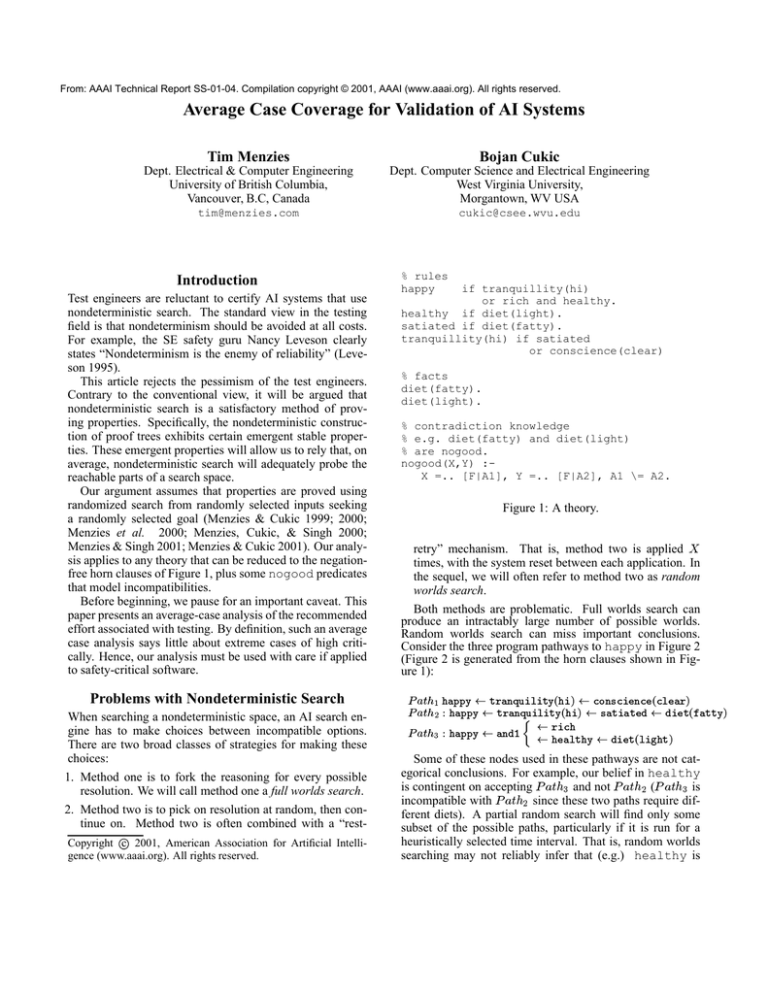
Figure 1: A theory.
retry” mechanism. That is, method two is applied times, with the system reset between each application. In
the sequel, we will often refer to method two as random
worlds search.
Both methods are problematic. Full worlds search can
produce an intractably large number of possible worlds.
Random worlds search can miss important conclusions.
Consider the three program pathways to happy in Figure 2
(Figure 2 is generated from the horn clauses shown in Figure 1):
"!# $%'& () &*&*+!,& *$
.-0/12 "!# $%3) * 44* +!65$
&;
"7/1'4"8:9 <* 124*"!=> $
Some of these nodes used in these pathways are not categorical conclusions. For example, our belief in healthy
is contingent on accepting ?A@BDC
E and not ?A@+BDCGF ( ?A@+BDCGE is
incompatible with ?A@+BDCGF since these two paths require different diets). A partial random search will find only some
subset of the possible paths, particularly if it is run for a
heuristically selected time interval. That is, random worlds
searching may not reliably infer that (e.g.) healthy is
Myes
M
Kand1 yesLrich
Myes H
10000
S=runtime (seconds)
Hhappy MyesItranquility(hi)
Oconscience(clear)
Myes
Myes
healthy
Myes J
diet(light)
Nsatiated
Myes J no
diet(fatty)
HT4
HT0
S=O(C^2)
1000
100
10
1
0.1
0
Figure 2: The rules of Figure 1 converted to an and-or graph.
All nodes here are or-nodes except and1. All parents of
an and-node must be believed if we are to believe and andnode. In this graph no-edges represent illegal pairs of inferences; i.e. things we can’t believe at the same time such as
diet(light) and diet(fatty). All other edges are
yes-edges which represent legal inferences.
Figure 3: HT4: full worlds search search- fork one world for
each consistent possibility reached from inputs. HT0: random worlds search- when contradictions are found, pick one
resolution at random, then continue. In the zone where both
algorithms terminated, HT0’s random world search found
98% of the goals found by HT4’s full worlds search.
ATMS system, a well-known full worlds search algorithm (Williams & Nayak 1996).
an uncertain conclusion. Depending on how the conflict
between diet(light) and diet(happy) is resolved
at runtime, this system will sometimes nondeterministically
conclude healthy and sometimes it won’t.
This toy example is a simple demonstrator for a problem that can get much more complicated. A linear-time
pre-processor could detect the presence of the incompatible facts diet(light) and diet(happy). However,
in larger systems, the sources of contradictions may not
detectable without actually executing the system. Sadly,
such executions may not reveal all the features of the theory. Gabow et.al. (Gabow, Maheshwari, & Osterweil 1976)
showed that building pathways across graphs with impossible pairs (e.g.the no-edges in Figure 2) is NP-hard for all but
the simplest graphs (a graph is very simple if it is very small,
or it is a simple tree, or it has a dependency networks with
out-degree PRQ ). Hence searching graphs like Figure 2 can
take exponential time and any practical proof procedure for
properties across Figure 2 must use an incomplete search.
Empirical Studies of Nondeterminism
One measure of the effectiveness of a search procedure is
its cover: the percentage of the provable goals found by a
search engine. Suppose that randomized world search covers as many goals as a full worlds search. Such a result
would be consistent with the claim that nondeterministic
search is an adequate method for proving properties.
There is some empirical evidence that randomized search
does indeed cover as well as full search.
S
S
For CNF representations, it is well established that random search with retries can demonstrate satisfiability in
theories too large for full search (Kautz & Selman 1996).
Williams and Nayak found that a random worlds search
algorithm performed as well as the best available
3000 6000 9000 120001500018000
C=number of clauses
S
S
Menzies, Easterbrook et.al. report experiments comparing random world search with full world search for requirements engineering. After millions of runs, they concluded that randomized world search found almost as
many goals in less time as full worlds search (Menzies
et al. 1999).
In other work, Menzies and Michael compared a full
worlds search search with a random worlds search. As
expected, the full worlds search ran slow ( TVU,WX1Y ) while
F
the random worlds search ran much faster ( TVU,Z Y ); see
Figure 3. What is more interesting is that, for problems where both search methods terminated, the random
worlds search found 98% of the goals found by the full
worlds search (Menzies & Michael 1999).
Theoretical Studies of Nondeterminism
The above case studies encourage a belief that nondeterminism can adequately sample a space. However, the external
validity of isolated case studies must be questioned. Before
we can trust nondeterministic search, we need to generalize
the above case studies to show that, on average, the cover is
not greatly effected by nondeterminancy.
One method of generalizing the above case studies is to
consider the assumptions within the worlds of belief generated by search theories such as Figure 1.
S
S
Given a model such as Figure 2 and a goal such as
happy, heuristic search builds pathways to those goals;
e.g. ?A@+BDC\[]]] ?A@+BDC
E .
Anything that has not been asserted as a fact is an assumption. No path can contain mutually exclusive assumptions
or contradict the goal; i.e. assuming ^ happy is illegal.
S
The generated pathways should be grouped together into
consistent subsets called worlds. Our example
maximal
_
generates two worlds: `bacd,e [ = f ?A@+BDC [g ?A@+BDC Eh and
`bacd,e F = f?A@+BDC [g ?A@+BDC Fh .
S A world contains what we can conclude from and-or
graphs. A goal is proved if it can be found in a world.
S Assuming randomized search, only some of the possible
paths will be found at runtime. At different runtimes, different paths and hence different worlds will be generated.
The nondeterministic testing problem can formalized as
follows. The results of testing a nondeterministic system are
untrustworthy when either:
1. Not enough worlds are generated to cover the range of
possible conclusions. This first case could arise from
heuristics that prune possible inferences at runtime. Such
heuristics are often used when generating pathways from
a space containing conflicts. Recall that search spaces like
Figure 2 contain pairs of conflicts: one such pair exists
for each no-edge. Recalling the above mentioned result
of (Gabow, Maheshwari, & Osterweil 1976) (i.e. building pathways across programs with impossible pairs of
nodes is NP-complete for all but the simplest programs),
we can formally declare that any practical system must
conduct an incomplete partial search of search spaces like
Figure 2.
2. Too many worlds are generated and we are swamped with
possibilities. This second case has often observed in research into qualitative reasoning. When all possible consequences of inputs are generated from a nondeterministic
space, a vast suite of possibilities can be generated. Taming this intractable branching of behaviors is a major focus of research into qualitative reasoning (Menzies et al.
2001).
Both problems are removed if the total number of possible
worlds is small. If so, then:
S All the possible conclusions can be reached by sampling
just a few worlds; i.e. problem #1 goes away.
S
A large number of worlds will not be possible; i.e. problem #2 goes away.
To prove that, on average, the total number of possible worlds is small, we need to categorize assumptions
into three important groups. Only one of these assumption
groupings will determines how many worlds are generated.
Some assumptions are dependent on other assumptions.
For example, in ?A@+BDC
E , the healthy assumptions depends
fully on diet(light). In terms of exploring all the effects of different assumptions, we can ignore the dependent
assumptions.
Another important category of assumptions are the assumptions that contradict no other assumptions. These noncontroversial assumptions are never at odds with other assumptions and so do not effect the number of worlds generated. In our example, the non-controversial assumptions are
everything except diet(light) and diet(healthy).
Hence, like the dependent assumptions, we will ignore these
non-controversial assumptions.
The remaining assumptions are the controversial, nondependent assumptions or funnel assumptions. These funnel assumptions control how all the other assumptions are
grouped into worlds of belief. DeKleer’s key insight in
the ATMS research was that a multi-world reasoning device need only focus on the funnel (DeKleer 1986)1. When
switching between worlds, all we need to resolve is which
funnel assumptions we endorse. Continuing our example,
if we endorse diet(light) then all the conclusions in
`bacd,eF follow and if we endorse diet(healthy) then
all the conclusions in `bacd,e [ follow.
Paths meet and clash in the funnel. If the size of the funnel
is very small, then the number of possible clashes is very
small and the number of possible resolutions to those clashes
is also very small. When the number of possible resolutions
is very small, the number of possible worlds is very small
and random search can quickly probe the different worlds of
beliefs (since there are so few of them). Hence, if we can
show that the average size of the funnel is small, then we
can quickly poll the range of possible conclusions from our
and-or graphs.
Average Funnel Size
Suppose some goal can be reached by a narrow funnel i
a wide funnel Z as follows:
l jjom nk i [
l
m p
i F
jl\om q ] ]]
ipr
~ttt
s ttu
v
or
tt
k
ttt Z[} l
n
tt
ZF} n l
l
myx a@"d6z|} { l ttt ZE} n l
ttt Z
} l
w
tt
]]]
}
Z l
We say that the probability of reaching the goal is the value
c@"C
e .
Under what circumstances will the narrow funnel be favored over the wide funnel? More precisely, when are the
odds of reaching x a@"d6z via the narrow funnel much greater
that the odds of reaching x a@"d z via the wide funnel? The
following analysis answers those questions using the framework of (Menzies & Singh 2001) (with less needless mathematical complexity and with a wider range of distributions
for the simulation studies).
To find the average funnel size, we begin with the following definitions. Let the i funnel use variables and the
Z funnel use variables. For comparison purposes, we express the size of the wider funnel as a ratio of the narrower
funnel; i.e.
(1)
Each member of i is reached via a path with probability @ z
while each member of Z is reached via a path with probability oz . Two paths exist from the funnels to this goal: one
1
DeKleer called the funnel assumptions the minimal environments. We do not adopt that terminology here since DeKleer used
consistency-based abduction while we are exploring set-covering
abduction here. For an excellent discussion that defines and distinguishes set-covering from consistency-based methods, see (Console & Torasso 1991).
from the narrow neck with probability and one from the
wide neck with probability e . The probability of reaching
the goal via the narrow pathway is
@+c ca
r
@z
z[
(2)
while the probability of reaching the goal via the wide pathway is
e+e
oz
z[
Let ?¡U¢@+cca£ c@"C
e+Y and ?¡U= e.£ c @"C
e+Y
(3)
denote
the conditional probabilities of using one of the funnels,
given that the goal is reached. The ratio ¤ of these conditional probabilities informs us when the narrow funnel is
favored over the wider funnel.
jo§¨§ª©D«
ª§ ¬­j ¬
@+c ca
« ¬ e+ (4)
§¥ ª¬­j zw { ® ¬ {.¯
{¯
Narrow funnels are more likely than
w ® wider funnels when
¤±°²Q .
To compute the frequency of ¤³°yQ , we have to make
? U=@cca£ c @"C
e+Y ¦¥
¤b ¡
? U¢ e+"£ c@+CGe"Y
¡
some assumptions about the probability distributions of
@+cca and c@+CGe . (Menzies & Singh 2001) showed that
if @ z and z come from uniform probability distributions,
then narrow funnels are more likely than wide funnels. In
the case of such uniform distributions,
´r
Q r
@+z±Qµ¶@+z· Q µ¶@+ccabA¸ º
¹
z[
(6)
(9)
Ï
j zj {DÒ
(10)
{
Ï
Ð
z is the probability we computed in the prior step of
where
being the base case). The probability
the simulation (and
of reaching an or-node with acªÑ parents is the probability of
not missing any of Ï its parents; i.e.: Ï
©À§ bQ l U­Q l
(7)
Consider the case of two funnels, one twice as big as the
other; i.e. ¶jo½
§¨§¨©ÀW « . This expression can then be rearranged to
show that « z ¬ °²Q is true when
{
Î
The probability of reaching an and-node with @eÑ parents
is the probability of reaching
allÏ its parents; i.e.
Ï
Under this assumption of uniformity, ¤±°½Q when
r
@+cca ¥ r [
e
e [ ¯
¥ ¯
Recalling that » , this expression becomes
U=¾YÀ¿ r ÂÁ r ° e
A Reachability Model
Menzies, Cukic, Singh and Powell (Menzies et al. 2000)
computed the odds of reaching some random part of a space
of nondeterminant choices from random inputs. The analysis assumed that software had been transformed into a possibly cyclic directed graph containing and-nodes and ornodes; e.g. Figure 1 has been converted to Figure 2. A
simplified description of their analysis is presented here. For
full details, including details such as using random variables
and testing for loops and contradictions, see (Menzies et al.
2000).
Assume that “ ” number of inputs have been presented
to a graph containing Î nodes. From these inputs, we grow
a tree of pathways down to some random node within the
graph. The odds of reaching a node straight away from the
inputs is
ÏGÐ
(5)
Similarly, under the same assumptions,
Q
e+1»e ¸ ¼
¹
assumptions of this uniform case, as the wide funnel gets
wider, it becomes less and less likely
that it will ber used.
r
To explore the case where Ê zË[ @ z¼b
Ì Q and Ê zË·[ z0
Ì Q
(i.e. the non-uniform probability distribution case), we created and executed a small simulator many times. In this simulator, we found the frequency at which ¤Í°B where B was
some threshold value.
To execute the simulator, we required some knowledge of
the distributions of @cca and e+ when they are computed by nondeterministic search.Those distributions were
taken from an average case analysis of reachability across
graphs such as Figure 2. This reachability analysis is discussed below.
U=ÃY r ° e
(8)
At ÄÅW , Equation 8 becomes eÆÇÃ . That is, to access x a@+d6z from the wider funnel, the pathway e must be
64 times more likely than the pathway . This is not highly
likely and this becomes less likely as the narrower funnel
grows. By the same reasoning, at È'É , to access x a@"d z
from the wider funnel, the pathway e must be 1728 times
more likely than the narrower pathway . That is, under the
©À§
zY Ò
(11)
If the ratio of and-nodes in a network is @+e Ó , then the ratio
ÏÔ
of or-nodes in the same network is Q l @+e Ó . The odds of
is the weighted sum of the
reaching some random node
Ï
Ï
probabilities ofÏ.Ôreaching and-nodes
or or-nodes;
i.e.
Ï Ô @+e Ó¡Õ j
{×Ö
acÓ¡Õ ©D§
Z ÏÔ
(12)
We can convert
to the number of tests
required to
as follows.
be 99% sure of find a fault with probability
Equation 11 is really the sampling-with-replacement equation where acªÑ is the number of trials Z . We can use
sampling-with-replacement to find the certainty of finding
some event after Z trials. If we demand a 99% certainty
of reaching a node at step Ø (i.e. Ù|ÚG] ÛÛ ), then we can
re-arrange Equation 11 to
Z
d,a x DU Q l ÚGÏ ] ÛÔ ÛY
d=a x U­Q l Y
(13)
t=1
% when R>t
After 150,000 simulations of this model, some best and
worst
Ü cases were identified. These are shown in Figure 4
labeled pessimistic and optimistic respectively. In the pessimistic case, we restricted the depth of our search to some
trivial size: ØÝÆÈQÚ . In this pessimistic case, more than
10,000 random inputs are required to reach half the nodes in
the graphs we simulated. In the optimistic case, we gave the
search engine greater freedom to explore: ØÞÆ<QÚÚ . In this
optimistic case, less than 100 random inputs would reach
over half the nodes in the graphs we simulated.
ó
100
80
60
40
20
0
pessimistic
optimistic
log normal
1
2
3
@+z g ;z g g e were taken from one of three distributions: the
pessimistic and optimistic curves shown in Figure 4, plus a
log normal curve (just for comparison purposes). For the
F
log-normal curve, mean ã and standard deviation ä of the
logarithm of the variables were picked at random from the
following ranges:
ã¶ßÞf+Q g W g ]]]oQÚ h ; åDÑ
c @"e¡ßÂf ÚG] Ú+â g Ú]Q g ÚG] W g ÚG] à g Ú] æ h
åÀÑ
c@"e
where then converted into probability as
[¨ç D© § r èéz#êëìËí+î ï n¨ð
ä F »åDÑ
c @"eÕ×ã
; Ñ
ca;@"od=B ÙbQÚ Á
¤ was then calculated and the number of times ¤ exceeded
different values for B is shown in Figure 5. As might be expected, at BébQ g ±Q the funnels are the same size and the
odds of using one of them is 50%. As increases, then increasingly ¤±°ñB is satisfied and the narrower funnel is preferred to the wider funnel. The effect is quite pronounced.
N (average)
1e+14
1e+6
10,000
100
1
j=1..10
0
25 50 75 100
%
N (average)
Optimistic:
ò
1e+14
1e+6
10,000
100
1
8
9
10
% when R>t
ó
100
80
60
40
20
0
8
9
10
pessimistic
optimistic
log normal
1
2
3
4
5
6
7
alpha
Figure 5: 10000 runs of the funnel simulator. Y-axis shows
what percentage of the runs satisfies ¤±°ºB .
For example, for all the studied distributions, if the wider
funnel is 2.25 times bigger than the narrow funnel, random
search will be 1,000,000 times as likely as to use the narrow funnel (see the lower graph of Figure 5). Interestingly,
as reachability drops, the odds of using the narrow funnel
increase (see the pessimistic curves in Figure 5). That is,
the harder the search, the less likely the search will suffer
from the problem of indeterminate search under-sampling
the space.
Discussion
1. The formal verification community seeks near-complete
inference procedures Our results assume random search
and random search is not attractive to proponents of complete search.
2. CNF-based theorem provers do not have a strong concept of a proof tree. Hence, the satisfiability community
would not have seen the above results since our analysis
requires knowledge of the traversal path taken from inputs
to goals.
j=91..100
0
7
Why have these optimistic average case results for nondeterministic search been reported before? Several research
communities might have seen the same results. However,
the premises of those communities may have blocked them
from finding these conclusions:
Pessimistic:
ò
6
t= 1,000,000
Having some knowledge of the distributions, we can now
compute the frequency of ¤|°RB for non-uniform distributions. For one run of the Equation 4 simulator, and were
picked at random from the ranges:
àßÂfQ g W g ]]]oQÚ h ; áßÂfQ g Q] Wâ g Q] â g ]]]¨QÚ h
and
follows:
5
alpha
Simulating Funnels
ã
4
25 50 75 100
%
ÏÔ
Figure 4: 150,000 runs of the simulator generated figures
which were converted into number of tests Z required using
Equation 13. X-axis shows the percentile distribution of the
output of the runs.
3. The software engineering (SE) testing community uses
procedural systems that take fixed pathways through their
systems. Our results assume that a test procedure can
take random detours during the test procedure. This is
not an acceptable procedure for most of the SE test community. However, amongst the small group of SE test researchers that conduct randomization studies of SE sys-
tem, some recent empirical results endorse our proposal
that
_ random search is an adequate test strategy (Horgan &
Mathur 1996).
Conclusion
It has been argued that for a wide range of distributions (uniform, pessimistic, optimistic, log-normal), random search
engines will favor worlds with narrow funnels. As funnel size grows, the number of different worlds also grows.
Hence, size the average funnel size is small, the number of
different worlds will also be small. Consequently:
S
S
On average, the impact on goal coverage due to nondeterminism is small.
Nondeterministic search is an adequate method for proving properties in a system.
Acknowledgments
Holgar Hoss’s comments on the maths of (Menzies & Singh
2001) prompted the simpler analysis shown here.
References
Console, L., and Torasso, P. 1991. A Spectrum of Definitions of
Model-Based Diagnosis. Computational Intelligence 7:133–141.
DeKleer, J. 1986. An Assumption-Based TMS. Artificial Intelligence 28:163–196.
Gabow, H.; Maheshwari, S.; and Osterweil, L. 1976. On two
problems in the generation of program test paths. IEEE Trans.
Software Engrg SE-2:227–231.
Horgan, J., and Mathur, A. 1996. Software testing and reliability. In Lyu, M. R., ed., The Handbook of Software Reliability
Engineering, 531–565.
Kautz, H., and Selman, B. 1996. Pushing the envelope: Planning, propositional logic and stochastic search. In Proceedings
of the Thirteenth National Conference on Artificial Intelligence
and the Eighth Innovative Applications of Artificial Intelligence
Conference, 1194–1201. Menlo Park: AAAI Press / MIT Press.
Available from http://www.cc.gatech.edu/˜jimmyd/
summaries/kautz1996.ps.
Leveson, N. 1995. Safeware System Safety And Computers.
Addison-Wesley.
Menzies, T., and Cukic, B. 1999. On the sufficiency of limited
testing for knowledge based systems. In The Eleventh IEEE International Conference on Tools with Artificial Intelligence. November 9-11, 1999. Chicago IL USA.
Menzies, T., and Cukic, B.
2000.
When to test less.
IEEE Software 17(5):107–112. Available from http://tim.
menzies.com/pdf/00iesoft.pdf.
Menzies, T., and Cukic, B. 2001. Submitted to Handbook of
Software Engineering and Knowledge Engineering, Volume II.
World-Scientific. chapter How Many Tests are Enough? Available from http://tim.menzies.com/pdf/00ntests.
pdf.
Menzies, T., and Michael, C. 1999. Fewer slices of pie: Optimising mutation testing via abduction. In SEKE ’99, June
17-19, Kaiserslautern, Germany. Available from http://tim.
menzies.com/pdf/99seke.pdf .
Menzies, T., and Singh, H. 2001. Many maybes mean (mostly)
the same thing. In Submitted to the 2nd International Workshop on Soft Computing applied to Software Engineering (Netherlands), February. Available from http://tim.menzies.
com/pdf/00maybe.pdf.
Menzies, T.; Easterbrook, S.; Nuseibeh, B.; and Waugh, S.
1999. An empirical investigation of multiple viewpoint reasoning in requirements engineering. In RE ’99. Available from
http://tim.menzies.com/pdf/99re.pdf.
Menzies, T.; Cukic, B.; Singh, H.; and Powell, J. 2000. Testing
nondeterminate systems. In ISSRE 2000. Available from http:
//tim.menzies.com/pdf/00issre.pdf.
Menzies, T.; Cohen, R.; Waugh, S.; and Goss, S. 2001. Applications of abduction: Testing very long qualitative simulations.
IEEE Transactions of Data and Knowledge Engineering (to appear). Available from http://tim.menzies.com/pdf/
97iedge.pdf.
Menzies, T.; Cukic, B.; and Singh, H. 2000. Agents talking
faster. NASA Goddard Workshop on Formal Aspects of AgentOriented Systems. Available from http://tim.menzies.
com/pdf/00godd.pdf.
Williams, B., and Nayak, P. 1996. A model-based approach to reactive self-configuring systems. In Proceedings, AAAI ’96, 971–
978.
