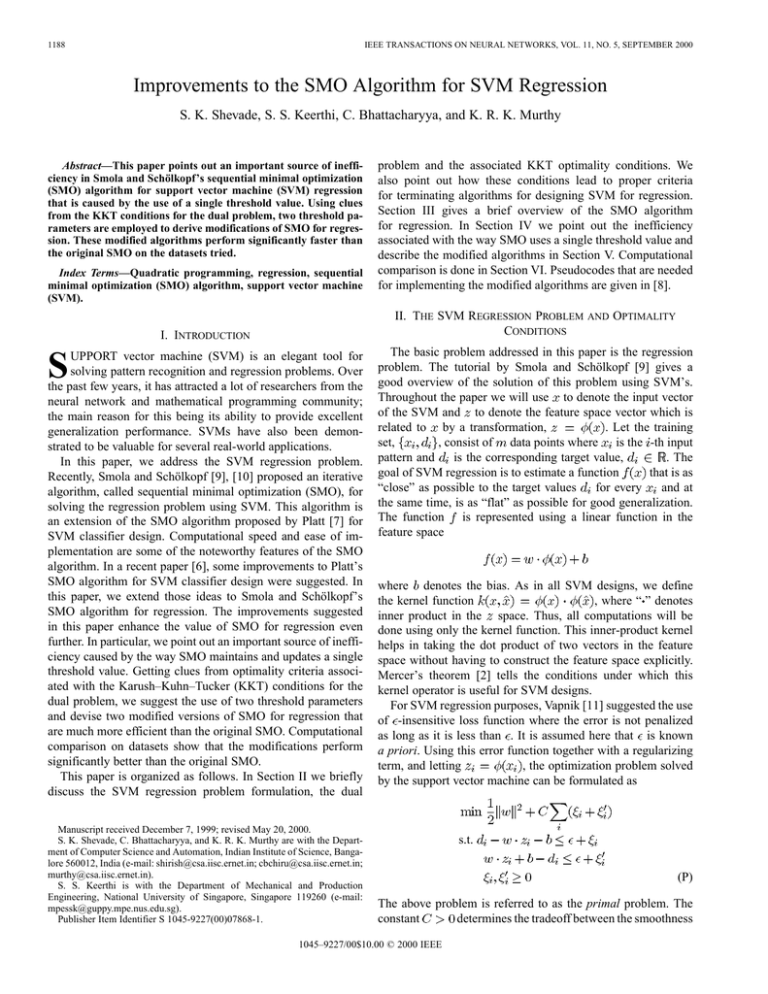
1188
IEEE TRANSACTIONS ON NEURAL NETWORKS, VOL. 11, NO. 5, SEPTEMBER 2000
Improvements to the SMO Algorithm for SVM Regression
S. K. Shevade, S. S. Keerthi, C. Bhattacharyya, and K. R. K. Murthy
Abstract—This paper points out an important source of inefficiency in Smola and Schölkopf’s sequential minimal optimization
(SMO) algorithm for support vector machine (SVM) regression
that is caused by the use of a single threshold value. Using clues
from the KKT conditions for the dual problem, two threshold parameters are employed to derive modifications of SMO for regression. These modified algorithms perform significantly faster than
the original SMO on the datasets tried.
Index Terms—Quadratic programming, regression, sequential
minimal optimization (SMO) algorithm, support vector machine
(SVM).
problem and the associated KKT optimality conditions. We
also point out how these conditions lead to proper criteria
for terminating algorithms for designing SVM for regression.
Section III gives a brief overview of the SMO algorithm
for regression. In Section IV we point out the inefficiency
associated with the way SMO uses a single threshold value and
describe the modified algorithms in Section V. Computational
comparison is done in Section VI. Pseudocodes that are needed
for implementing the modified algorithms are given in [8].
II. THE SVM REGRESSION PROBLEM
CONDITIONS
I. INTRODUCTION
S
UPPORT vector machine (SVM) is an elegant tool for
solving pattern recognition and regression problems. Over
the past few years, it has attracted a lot of researchers from the
neural network and mathematical programming community;
the main reason for this being its ability to provide excellent
generalization performance. SVMs have also been demonstrated to be valuable for several real-world applications.
In this paper, we address the SVM regression problem.
Recently, Smola and Schölkopf [9], [10] proposed an iterative
algorithm, called sequential minimal optimization (SMO), for
solving the regression problem using SVM. This algorithm is
an extension of the SMO algorithm proposed by Platt [7] for
SVM classifier design. Computational speed and ease of implementation are some of the noteworthy features of the SMO
algorithm. In a recent paper [6], some improvements to Platt’s
SMO algorithm for SVM classifier design were suggested. In
this paper, we extend those ideas to Smola and Schölkopf’s
SMO algorithm for regression. The improvements suggested
in this paper enhance the value of SMO for regression even
further. In particular, we point out an important source of inefficiency caused by the way SMO maintains and updates a single
threshold value. Getting clues from optimality criteria associated with the Karush–Kuhn–Tucker (KKT) conditions for the
dual problem, we suggest the use of two threshold parameters
and devise two modified versions of SMO for regression that
are much more efficient than the original SMO. Computational
comparison on datasets show that the modifications perform
significantly better than the original SMO.
This paper is organized as follows. In Section II we briefly
discuss the SVM regression problem formulation, the dual
Manuscript received December 7, 1999; revised May 20, 2000.
S. K. Shevade, C. Bhattacharyya, and K. R. K. Murthy are with the Department of Computer Science and Automation, Indian Institute of Science, Bangalore 560012, India (e-mail: shirish@csa.iisc.ernet.in; cbchiru@csa.iisc.ernet.in;
murthy@csa.iisc.ernet.in).
S. S. Keerthi is with the Department of Mechanical and Production
Engineering, National University of Singapore, Singapore 119260 (e-mail:
mpessk@guppy.mpe.nus.edu.sg).
Publisher Item Identifier S 1045-9227(00)07868-1.
AND
OPTIMALITY
The basic problem addressed in this paper is the regression
problem. The tutorial by Smola and Schölkopf [9] gives a
good overview of the solution of this problem using SVM’s.
Throughout the paper we will use to denote the input vector
of the SVM and to denote the feature space vector which is
. Let the training
related to by a transformation,
, consist of data points where is the -th input
set,
is the corresponding target value,
. The
pattern and
that is as
goal of SVM regression is to estimate a function
for every
and at
“close” as possible to the target values
the same time, is as “flat” as possible for good generalization.
The function is represented using a linear function in the
feature space
where denotes the bias. As in all SVM designs, we define
, where “ ” denotes
the kernel function
inner product in the space. Thus, all computations will be
done using only the kernel function. This inner-product kernel
helps in taking the dot product of two vectors in the feature
space without having to construct the feature space explicitly.
Mercer’s theorem [2] tells the conditions under which this
kernel operator is useful for SVM designs.
For SVM regression purposes, Vapnik [11] suggested the use
of -insensitive loss function where the error is not penalized
as long as it is less than . It is assumed here that is known
a priori. Using this error function together with a regularizing
, the optimization problem solved
term, and letting
by the support vector machine can be formulated as
s.t.
(P)
The above problem is referred to as the primal problem. The
determines the tradeoff between the smoothness
constant
1045–9227/00$10.00 © 2000 IEEE
IEEE TRANSACTIONS ON NEURAL NETWORKS, VOL. 11, NO. 5, SEPTEMBER 2000
of and the amount up to which deviations larger than are
tolerated.
. We will refer to
Let us define
as Lagrange multipliers. Using Wolfe duality theory, it
the
are obtained by solving the following
can be shown that the
Dual problem:
1189
Case 1)
(1a)
Case 2)
(1b)
Case 3)
(1c)
s.t.
Case 4)
(D)
and
are obtained, the primal variables,
Once the
and can be easily determined by using the KKT conditions
for the primal problem.
The feature space (and hence ) can be infinite dimensional. This makes it computationally difficult to
solve the primal problem (P). The numerical approach
in SVM design is to solve the dual problem since it
is a finite-dimensional optimization problem. (Note that
.) To
derive proper stopping conditions for algorithms which solve
the dual, it is important to write down the optimality conditions
for the dual. The Lagrangian for the dual is
(1d)
Case 5)
(1e)
Define the following index sets at a given :
. Also,
let
. Let us also define
and
as
if
if
and
if
if
Using these definitions we can rewrite the necessary conditions
mentioned in (1a)–(1e) as
(2)
Let
It is easily seen that the optimality conditions will hold iff
there exists a satisfying (2).
Let us define
The KKT conditions for the dual problem are
(3)
Then the optimality conditions will hold at some
iff
(4)
These conditions are both necessary and sufficient for optimality. Hereafter, we will refer to them as optimality conditions.
These optimality conditions can be simplified by considering
the following five cases. It is easy to check that at optimality,
and
cannot be nonzero at the same time.
for every
have been left out.
Hence cases corresponding to
(It is worth noting here that in the SMO regression algorithm
and its modifications discussed in this paper, the condition,
is maintained throughout.)
There exists a close relationship between the threshold parameter in the primal problem and the multiplier, . The KKT
conditions of the primal (P) and dual (D) problem imply that,
at optimality, and are identical. This can be seen from the
following: 1) setting the derivative of the Lagrangian of (P) with
respect to to zero gives the equality constraint in (D) and 2) in
, is the Lagrangian multiplier of that equality constraint;
and hence, at optimality and coincide. Therefore, in the rest
of the paper, and will denote one and the same quantity.
defines a violation at
We will say that an index pair
if one of the following two sets of conditions holds:
and
(5a)
and
(5b)
1190
IEEE TRANSACTIONS ON NEURAL NETWORKS, VOL. 11, NO. 5, SEPTEMBER 2000
Note that optimality condition will hold at iff there does not
that defines a violation.
exist any index pair
Since, in numerical solution, it is usually not possible to
achieve optimality exactly, there is a need to define approximate
optimality conditions. The condition (4) can be replaced by
(6)
where is a positive tolerance parameter. (In the pseudocodes
given in [8], [10], this parameter is referred to as tol). Correspondingly, the definition of violation can be altered by replacing (5a) and (5b), respectively, by
and
(7a)
and
(7b)
Hereafter in the paper, when optimality is mentioned it will
mean approximate optimality.
Let
Using (1) it is easy to check that optimality holds iff there exists
a such that the following hold for every :
(8a)
(8b)
(8c)
(8d)
These conditions are used in [9], [10] together with a special
choice of to check if an example violates the KKT conditions.
However, unless the choice of turns out to be right, using the
above conditions for checking optimality can be incorrect. We
will say more about this in Section IV after a brief discussion of
Smola and Schölkopf’s SMO algorithm in the next section.
It is also possible to give an alternate approximate optimality
condition based on the closeness of the dual objective function
to the optimal value, estimated using duality gap ideas. This is
fine, but care is needed in choosing the tolerance used; see [5]
for a related discussion. This criterion has the disadvantage that
it is a single global condition involving all . On the other hand,
(7) consists of an individual condition for each pair of indexes
and hence is much better suited for the methods discussed in
satisfies (7) then a strict
this paper. In particular, when
improvement in the dual objective function can be achieved by
optimizing only the Lagrange multipliers corresponding to the
.)
examples and . (This is true even if
III. SMOLA
AND
SCHÖLKOPF’S SMO ALGORITHM
REGRESSION
FOR
A number of algorithms have been suggested for solving the
dual problem. Smola and Schölkopf [9], [10] give a detailed
view of these algorithms and their implementations. Traditional
quadratic programming algorithms such as interior point algorithms are not suitable for large size problems because of the
following reasons. First, they require that the kernel matrix be
computed and stored in memory. This requires extremely large
memory. Second, these methods involve expensive matrix operations such as Cholesky decomposition of a large submatrix of
the kernel matrix. Third, coding of these algorithms is difficult.
Attempts have been made to develop methods that overcome
some or all of these problems. One such method is chunking.
The idea here is to operate on a fixed size subset of the training
set at a time. This subset is called the working set and the optimization subproblem is solved with respect to the variables
corresponding to the examples in the working set and a set of
support vectors for the current working set is found. These current support vectors are then used to determine the new working
set. This new set is nothing but a set of worst input data points
which violate the optimality conditions for the current estimator.
The new optimization subproblem is solved and this process is
repeated until the optimality conditions are satisfied for all the
examples.
Platt [7] proposed an algorithm, called SMO for the SVM
classifier design. This algorithm puts chunking to the extreme
by iteratively selecting working sets of size two and optimizing
the target function with respect to them. One advantage of using
working sets of size two is that the optimization subproblem can
be solved analytically. The chunking process is repeated till all
the training examples satisfy the optimality conditions. Smola
and Schölkopf [9], [10] extended these ideas for solving the regression problem using SVM’s. We describe this algorithm very
briefly below. The details, together with a pseudocode can be
found in [9], [10]. We assume that the reader is familiar with
them. To convey our ideas compactly we employ the notations
used in [9], [10].
The basic step in the SMO algorithm consists of choosing a
and optimizing the dual objective funcpair of indexes,
tion in (D) by varying the Lagrange multipliers corresponding
to and only. We make one important comment here on the
role of the threshold parameter, . As in [9], [10] and in Secdenote the output error on the th pattern. Let us
tion II, let
call the indices of the two multipliers chosen for joint optimization in one step as and . To take a step by varying the Lagrange multipliers of examples and , we only need to know
. Therefore a knowledge of the value of
is not needed to take a step.
The method followed to choose and at each step is crucial for finding the solution of the problem efficiently. The SMO
algorithm employs a two loop approach: the outer loop chooses
; and, for a chosen the inner loop chooses . The outer loop
iterates over all patterns violating the optimality conditions,
first only over those with Lagrange multipliers neither on the
upper nor on the lower boundary (in Smola and Schölkopf’s
),
pseudocode this looping is indicated by
and once all of them are satisfied, over all patterns violating the
to ensure that the
optimality conditions
problem has indeed been solved. For efficient implementation
is maintained and updated for those indices
a cache for
corresponding to nonboundary Lagrange multipliers. The
are computed as and when needed.
remaining
Let us now see how the SMO algorithm chooses . The aim
is to make a large increase in the objective function. Since it is
IEEE TRANSACTIONS ON NEURAL NETWORKS, VOL. 11, NO. 5, SEPTEMBER 2000
expensive to try out all possible choices of and choose the
one that gives the best increase in the objective function, the
or
index is chosen to maximize
depending on the multipliers of and . Since
is available
in cache for nonboundary multiplier indexes, only such indexes
are initially used in the above choice of . If such a choice of
does not yield sufficient progress, then the following steps
are taken. Starting from a randomly chosen index, all indexes
corresponding to nonbound multipliers are tried as a choice for
, one by one. If still sufficient progress is not possible, all
indexes are tried as choices for , one by one, again starting
from a randomly chosen index. Thus the choice of random seed
affects the running time of SMO.
Although a value of is not needed to take a step, it is needed
if (8a)–(8d) are employed for checking optimality. In the SMO
algorithm is updated after each step. A value of is chosen so
. If, after a step involving
,
as to satisfy (1) for
(or both) takes a nonboundary value then (1d) or
one of
(1e) is exploited to update the value of . In the rare case that this
,
does not happen, there exists a whole interval, say,
of admissible thresholds. In this situation SMO simply chooses
to be the midpoint of this interval.
IV. INEFFICIENCY OF THE SMO ALGORITHM
The SMO algorithm for regression, discussed above, is
very simple and easy to implement. However it can become
inefficient because of its way of computing and maintaining a
single threshold value. At any instant, the SMO algorithm fixes
based on the current two indexes used for joint optimization.
However, while checking whether the remaining examples
violate optimality or not, it is quite possible that a different,
may do a better job. So, in the SMO
shifted choice of
has
algorithm it is quite possible that, even though
reached a value where optimality is satisfied (i.e., (6)), SMO
has not detected this because it has not identified the correct
choice of . It is also quite possible that, a particular index
may appear to violate the optimality conditions because (8) is
employed using an “incorrect” value of although this index
may not be able to pair with another to make progress in the
objective function. In such a situation the SMO algorithm does
an expensive and wasteful search looking for a second index
so as to take a step. We believe that this is a major source of
inefficiency in the SMO algorithm.
There is one simple alternate way of choosing that involves
all indices. By duality theory, the objective function value in
(P) of a primal feasible solution is greater than or equal to the
objective function value in (D) of a dual feasible solution. The
difference between these two values is referred to as the duality
gap. The duality gap is zero only at optimality. Suppose
is given and
. For each , the term can be chosen
optimally (as a function of ). The result is that the duality gap
is expressed as a function of only. One possible way of improving the SMO algorithm is to always choose so as to minimize the duality gap. This corresponds to the subproblem
1191
The solution of this subproblem is easy. Let
denote the
number of examples. In an increasing order arrangement of
and
let and
be the th and
-th
values. The function optimized in the above minimization
problem is a convex function of . The slope of this convex
values smaller than
, it is
function is negative at all
and it is zero for
positive at all values bigger than
. Therefore any in the interval,
is
and
can be done
a minimizer. The determination of
efficiently using a “median-finding” technique. Since all
are not typically available at a given stage of the algorithm,
it is appropriate to apply the above idea to that subset of
are available. This set contains .
indexces for which
We implemented this idea and tested it on some benchmark
problems. The idea led to a reasonable improvement over the
original SMO. However the modifications that we suggest in
the next section gave much greater improvements. See Section
VI for performances on some examples.
V. MODIFICATIONS OF THE SMO ALGORITHM
In this section, we suggest two modified versions of the SMO
algorithm for regression, each of which overcomes the problems
mentioned in the last section. As we will see in the computational evaluation of Section VI, these modifications are always
better than the original SMO algorithm for regression and in
most situations, they also give quite a remarkable improvement
in efficiency.
In short, the modifications avoid the use of a single threshold
value and the use of (8) for checking optimality. Instead, two
and
are maintained and (6) (or
threshold parameters,
(7)) is employed for checking optimality. Assuming that the
reader is familiar with [9] and the pseudocodes for SMO given
there, we only give a set of pointers that describe the changes
that are made to Smola and Schölkopf’s SMO algorithm for regression. Pseudocodes that fully describe these can be found in
[8].
is available for all . Let
1) Suppose, at any instant,
and
be indices such that
(9a)
and
(9b)
Then checking a particular for optimality is easy. For example,
. We only have to check if
. If this
suppose
condition holds, then there is a violation and in that case SMO’s
.
takeStep procedure can be applied to the index pair
Similar steps can be given for indexes in other sets. Thus, in
our approach, the checking of optimality of the first index,
and the choice of second index, , go hand in hand, unlike the
original SMO algorithm. As we will see below, we compute and
and
via an efficient updating process.
use
2) To be efficient, we would, like in the SMO algorithm,
; cache for
spend much of the effort altering
are maintained and updated to do this efficiently. And, when op, only then all indices are examined
timality holds for all
for optimality.
1192
3) The procedure takeStep is modified. After a successful
, let
. We
step using a pair of indices,
and
using only (i.e.,
compute, partially,
in (9)). Note that these extra steps are inexpenuse only
is available and updates of
sive because cache for
are easily done. A careful look shows that, since and
have been just involved in a successful step, each of the two
and
, is nonempty; hence
sets,
and
will not be null
the partially computed
and
could take values from
and
elements. Since
they are used as choices for in the subsequent step (see item
and
also in cache.
1 above), we keep the values of
, i.e., a loop with
4) When working with only
, one should note that, if (6) holds at some
is conpoint then it implies that optimality holds as far as
cerned. (This is because, as mentioned in item 3 above, the
and
are influenced by all indexes in .) This
choice of
gives an easy way of exiting this loop.
5) There are two ways of implementing the loop involving
.
indexes in only
Method 1: This is similar to what is done in SMO. Loop
. For each , check optimality and if violated,
through all
then
choose appropriately. For example, if
.
there is a violation and in that case choose
Method 2: Always work with the worst violating pair, i.e.,
and
.
choose
Depending on which one of these methods is used, we call
the resulting overall modification of SMO as SMO-Modification 1 and SMO-Modification 2. SMO and SMO-Modification
1 are identical except in the way optimality is tested. On the
other hand, SMO-Modification 2 can be thought of as a further
improvement of SMO-Modification 1 where the cache is effec.
tively used to choose the violating pair when
holds, as already said we come
6) When optimality on
.
back to check optimality on all indexes
Here we loop through all indexes, one by one. Since
and
have been partially computed using only, we
update these quantities as each is examined. For a given
is computed first and optimality is checked using the current
and
; if there is no violation,
are used
and
to update these quantities. For example, if
, then there is a violation, in which case we take a step
. On the other hand, if there is no violation, then
using
is modified using , i.e., if
then we do:
and
.
7) Suppose we do as described above. What happens if there
? Can
is no violation for any in a loop having
we conclude that optimality holds for all ? The answer to this
question is affirmative. This is easy to see from the following
argument. Suppose, by contradiction, there does exist one
pair such that they define a violation, i.e., they satisfy (7). Let
. Then would not have satisfied the optimality
us say,
check in the above described implementation because either
or
would have, earlier than is seen, affected either the caland/or
settings. In other words, even if
culation of
is mistakenly taken as having satisfied optimality earlier in the
loop, will be detected as violating optimality when it is analyzed. Only when (6) holds it is possible for all indices to satisfy
IEEE TRANSACTIONS ON NEURAL NETWORKS, VOL. 11, NO. 5, SEPTEMBER 2000
Fig. 1. Toy data: CPU time (in seconds) shown as a function of C .
the optimality checks. Furthermore, when (6) holds and the loop
and
over all indices has been completed, the true values of
, as defined in (3) would have been computed since all indices have been encountered. As a final choice of (for later use
.
in doing inference) it is appropriate to set:
VI. COMPUTATIONAL COMPARISON
In this section we compare the performance of our modifications against Smola and Schölkopf’s SMO algorithm for regression and the SMO algorithm based on duality gap ideas for
threshold (see Section IV), on three datasets. We implemented
all these methods in C and ran them using gcc on a P3 450
was used for all exMHz Linux machine. The value,
periments. For every dataset used in the experiments, we added
an independent Gaussian noise of mean zero and some standard
deviation. For every dataset, the value of was manually set in
a random way depending upon the amount of noise added to the
data. Similar experimental approaches include [4]. The input as
well as the output are then normalized so as to have zero mean
and a unit variance.
The first dataset is a toy dataset where the function to be ap. The doproximated is a cubic polynomial,
main of this function was fixed to [ 10, 10]. The value,
was used. One hundred training samples were chosen randomly. The performance of the four algorithms for the polynomial kernel
where was chosen to be three (the degree of the polynomial
from which the data is generated), is shown in Fig. 1.
The second dataset is the Boston housing dataset which is
a standard benchmark for testing regression algorithms. This
dataset is available at UCI Repository [1]. The dimension of the
input is 13. We used a training set of size 406. The value,
was used. Fig. 2 shows the performance of the four algorithms
on this dataset. For this as well as the third dataset the Gaussian
kernel
IEEE TRANSACTIONS ON NEURAL NETWORKS, VOL. 11, NO. 5, SEPTEMBER 2000
1193
ciency is remarkable. In particular, at large values of the improvement is by an order of magnitude. Between the two modifications, it is difficult to say which one is better.
The primary purpose of these experiments is to examine differences in training times of all the four methods. However,
studying the generalization abilities of these methods is an important task and we are currently investigating it. The results of
this comparison will be reported elsewhere.
VII. CONCLUSION
Fig. 2. Boston housing data: CPU time (in seconds) shown as a function of C .
In this paper, we have pointed out an important source of
inefficiency in Smola and Schölkopf’s SMO algorithm that is
caused by the operation with a single threshold value. We have
suggested two modifications of the SMO algorithm that overcome the problem by efficiently maintaining and updating two
threshold parameters. Our computational experiments show that
these modifications speed up the SMO algorithm significantly
in most situations. The modifications can be easily implemented
using the pseudocodes given in [8].
REFERENCES
Fig. 3. Comp-Activ data: CPU time (in seconds) shown as a function of C .
was used and the
value employed was 2.5. The value of
was chosen randomly. The SVM is rather insensitive to different
choices of .
The third dataset, Comp-Activ, is available at the Delve website [3]. This dataset contains 8192 data points of which we
used 5764. We implemented the “cpuSmall” prototask, which
involves using 12 attributes to predict the fraction of time (in
for this
percentage) the CPU runs in user mode. We used
dataset. The performance of the four algorithms on this dataset
is shown in Fig. 3.
It is very clear that both modifications outperform the original
SMO algorithm. In many situations the improvement in ef-fi-
[1] C. L. Blake and C. J. Merz. (1998) UCI Repository of Machine
Learning Databases. Univ. California, Dept. Inform. Comput. Sci.,
Irvine, CA. [Online]. Available: http://www.ics.uci.edu/~mlearn/MLRepository.html
[2] C. J. C. Burges, “A tutorial on support vector machines for pattern recognition,” Data Mining Knowledge Discovery, vol. 3, no. 2, 1998.
[3] Delve: Data for Evaluating Learning in Valid Experiments [Online].
Available: http://www.cs.utoronto.ca/~delve
[4] O. L. Mangasarian and D. R. Musicant. (1999, Aug.)
Massive Support Vector Regression. [Online] . Available:
ftp://ftp.cs.wisc.edu/pub/dmi/tech-reports/99-02.ps
[5] S. S. Keerthi, S. K. Shevade, C. Bhattacharyya, and K. R. K. Murthy, “A
fast iterative nearest point algorithm for support vector machine classifier design,” IEEE Trans. Neural Networks, vol. 11, pp. 124–136, Jan.
2000.
, (1999, Aug.) Improvements to Platt’s SMO Algorithm for SVM
[6]
Classifier Design, Accepted for Publication in Neural Computation.
Control Division, Dept. of Mechanical and Production Engineering,
National University of Singapore, Singapore. [Online]. Available:
http://guppy.mpe.nus.edu.sg/~mpessk
[7] J. C. Platt, Advances in Kernel Methods: Support Vector Machines,
B. Schölkopf, C. Burges, and A. Smola, Eds. Cambridge, MA:
MIT Press, Dec. 1998. Fast training of support vector machines using
sequential minimal optimization.
[8] S. K. Shevade, S. S. Keerthi, C. Bhattacharyya, and K. R. K. Murthy.
(1999, Aug.) Improvements to SMO Algorithm for Regression.
Control Division, Dept. of Mechanical and Production Engineering,
National University of Singapore, Singapore. [Online]. Available:
http://guppy.mpe.nus.edu.sg/~mpessk
[9] A. J. Smola, “Learning with Kernels,” Ph.D. dissertation, GMD, Birlinghoven, Germany, 1998.
[10] A. J. Smola and B. Schölkopf, “A Tutorial on Support Vector Regression,” Royal Holloway College, London, U.K., NeuroCOLT Tech. Rep.
TR 1998-030, 1998.
[11] V. Vapnik, The Nature of Statistical Learning Theory. New York:
Springer-Verlag, 1995.