From: AAAI Technical Report SS-94-05. Compilation copyright © 1994, AAAI (www.aaai.org). All rights reserved.
Geometric
Image Analysis
Using
Multiscale
Statistical
Features
James M. Coggins and Elizabeth Graves
Department of Computer Science
University of North Carolina at Chapel Hill
Iany medical image analysis problems involve
ixel classification tasks such as segmentation and
mdmarkidentification. This paper describes a
lethodology for defining an optimal feature space
~r performing such tasks based on a principled,
~neralized image decomposition. The methodology
;demonstrated on two kinds of test images, and
le nature of the optimization is illustrated.
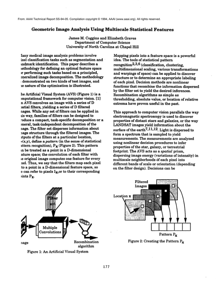
he Artificial Visual System(AVS)(Figure 1)
~mputational frameworkfor computer vision. [1]
n AVSconvolves an image with a series of D
mtial filters, yielding a series of Dfiltered
aages. Whileany set of filters can be applied in
ds way, families of filters can be designed to
.~oduce a compact, task-specific decompositionor a
meral, task-independent decomposition of the
aage. The filter set disperses information about
.~age structure through the filtered images. The
~tputs of the filters at a particular location,
=(x,y), define pattern (i n the sense ofstatistical
lttern recognition), Px (Figure 2). This pattern
m be treated as a point in a D-dimensional
ature space; the convolution of each filter with
Le original image computesone feature for every
xel. Thus, we say that the filters mapeach pixel
to a point in a D-dimensionalfeature space, so
e can refer to pixels Ix, or to their corresponding
~ints Px.
Mappingpixels into a feature space is a powerful
idea. Thetools of statistical pattern
recognition2,3,6 (classification, clustering,
multidimensional scaling, various transformations
and warpings of space) can be applied to discover
structure or to determine an appropriate labeling
of each pixel. Decision methods are nonlinear
functions that recombine the information dispersed
by the filter set to yield the desired inferences.
Recombination algorithms as simple as
thresholding, absolute value, or location of relative
extrema have proven useful in the past.
This approach to computer vision parallels the way
electromagnetic spectroscopy is used to discover
properties of distant stars and galaxies, or the way
LANDSAT
images yield information about the
surface of the earth7,11,12. Light is dispersed to
form a spectrum that is sampled to yield
measurements. The measurements are analyzed
using nonlinear decision procedures to infer
properties of the star, galaxy, or terrestrial
footprint. The AVSacts as a spatial prism,
dispersing image energy (variations of intensity)
multiscale neighborhoodsof each pixel into
different bands of scale or orientation (depending
on the filter design). Decisions can be
Filtered
Images
Location x
Multiple
Convolutions
Pattern Px
Figure 2: Creating the Pattern Px
Recombination
algorithm
Figure 1: An Artificial Visual System
aage
177
madeabout the objects portrayed in the image
based on nonlinear processing of the patterns Px.
This approach reveals a unified, coherent vision for
computer vision:
computer vision is spatial spectroscopy.
Our goal is to define a unified, scientific foundation
for computer vision based on spatial spectroscopy
and to develop methods for engineering AVS-like
systems to solve practical (mostly biomedical)
problems(see also [2]).
Structural Descriptionsof Images
An image is an uninterpreted recording of
intensity. The interpretation of image content
begins with a description of image structure. The
description of image structure produced by an AVS
is governedby the filter set. Filter sets for an AVS
can be defined ad hoc based on an understanding
of the task to be performed, but our experience
suggests that intuition misses subtleties that a
more principled approach can capture. A more
general, principled mechRnismfor defining the
filter set derives from a general, differential
geometric analysis of image structure.
Koenderink7,8,9 has defined several sets of
operators based on the Taylor Series expansion of
the local structure of an image,
Expanding
thebinomial
in (1)yields
theCartesian
family
of solutions.
Koenderink
alsodefines
a polar
family
anda "wavelet"
family.
Theith-order
derivatives
in anyoneof thesefamilies
canbe
linearly
combined
to formtheith-order
derivatives
oftheother
families.
To use these families of operators to describe
imagestructure requires definition of filter kernels
for each operator at each scale of interest. To
measure through 3rd-order derivatives at a series
of 6 scales requires 60 filter kernels. While
Koenderink’sreceptive field families yield a
complete geometric description of the intensity
structure, it is expensive to perform so many
convolutions, and with such a large number of
correlated features, the metric to use for
measuring distances in the feature space is
unclear.
An approximation to the Gaussian derivative
kernels yield tremendous computational savings.
Convolvingmultiscale Gaussian filters G(¢~) with
an image I and recording in Px the filter outputs at
x and at certain nearby locations, x+Si we obtain a
pattern that is related to Koenderink°spolar
operator family. The pattern is given formally by
Px = [I*G(~i)](x+Sij), 0_<i<S, 0<j<H
OO
where I is the image, G(~) is a Gaussian and
indexes the scales used in a decomposition, x is the
dx dy "
.=o
pixel location, and 8i] is the jth displacement
vector for the ith scale. The displacement vectors
¯ whereL(x,~) is the intensity of the image
we are using are oriented in the eight compass
location x=[x,y] aider convolution with a Gaussian
directions, and their lengths are related to the
with standard deviation ¢~. For the description of
standard deviation of the Gaussian. Since the
an image to introduce no spurious structure as the
feature
vector
incorporates
responses
to Gaussians
scale of measurementis enlarged, the resolution
at multiple
scales
andat multiple
nearby
locations,
kernel must be a solution to the diffusion equation,
thefeature
vector
at a particular
location
captures
d2f
df
imagestructure
across
spaceandscale.
d-~-~--~= 0.
Approximations
to Koenderink’s
generic
TheGaussian
is theGreen’s
function
(impulse
neighborhood
operators
arelinear
combinations
of
response
function)
of thediffusion
equation.
These
theseGaussians
andoffset
Gaussians.
(For
considerations
leadtotheuseofderivatives
of
example,
theLaplacian
is approximated
by a
Gaussians
as thesetoffilter
kernels
thatproduce
difference
of centered
Gaussians
at different
general
descriptions
of imagestructure.
The
scales.)
Thus,approximations
to manyof the
variance
of theGaussian
selects
thescaleof
derivative
of Gaussian
operators
arepresent
as
measurement,
andthederivatives
select
structural linesin theGaussian/offset
Gaussian
feature
features
oftheintensity
function.
Inpractice,
the
space.
Taylor
series
mustbe truncated.
Truncating
the
series
after
including
allderivatives
ofsome
Computationally, we can perform k convolutions
integral
order
results
ina representation
that
with Gaussians and extract up to 9 values (at
retains
thedesired
invariances.
Thistruncated
plus at offsets in the eight compassdirections at
series
iscalled
theN-jet
oftheimage
function.
distance kc) from each filtered image to obtain 9k
Thereare(N+1)(N+2)/2
kernels
in theN-jet.
178
~easurementsthat capture the (k-2)-jet across
tales. In fact, weget both moreand less than the
~-2)-jet. Somehigher-order structure is accessible
the feature space since k scales are measured,
ut someof the low-order "propeller" patterns are
ot well-captured by these particular offset
laussians. Thus, the feature set is not quite
rientation-invariant.
space. A different probability density must be
used, or the class must be split into components
better matched to a multivariate Gaussian. For
example, Gaussian mixture densities may provide
improvedfit at low computational cost.
Giventhe Gaussian fit for each class, we can
compute the Hotelling matrix, H=SBSw"
1, where
SB is the scatter matrix of the centroids (the
Scatter Between) and SWis the pooled scatter
matrix of the classes (Scatter Within) [4].
scatter matrix S is n~ for the set ofn points.) The
Hotelling Trace, J=trace(H), is a measure of the
separation between multivariate Gaussian
densities that is related to the probability of error
that would be obtained using an optimal linear
classifier [5]. It can be thought of as a multivariate
signal-to-noise ratio. The value of J increases with
larger separation between the classes and
decreases with larger variances in the classes. J is
highest, then, for compact,isolated clusters.
ComputingJ for manyclasses together gives an
averaged measure of "clustering tendency" in the
whole data set, but as averages often do, presents
a less than complete picture of the class structure.
Exploringthe FeatureSpace
n experiment begins by labeling regions in the
nage to define each class. Manysuch labelings
re possible on a given image. The labelings of
,ost interest for this exploration involve class
istinctions that are inherently geometric in
ature. Point operations are insufficient to
istinguish the classes. Part of the objective of this
.~dy is to begin characterizing classes that
;quire higher-order geometric measures to
istinguish the classes and thereby to begin
aswering the feature selection question: Of the
tony features available in the N-jet, whichones
re most relevant for the defined task? See [1].for
rumples of simpler geometric discriminations.
ll pixels are mappedto the feature space defined
3 Gaussian blurs and 5 spatial offsets. The
xels for each class form clouds in the feature
)ace. The cloud of points for class c can be
laracterized by its meanvector (centroid) ~c and
s covariance matrix Yc. For an arbitrary pixel x,
te Mahalanobisdistance of that pixers pattern Px
. the Gaussian density representring class c is
T.
d(x,c) = (Px-~c)Y’c’l(Px-I~c)
he covariance matrix, and thus the Mahalanobis
stance, account for the different variances of the
attires and for their correlations. Thevalue of
x,c) is a probability-normalized, squared distance
om the (hyperellipsoidal) multivariate Gaussian
2.
oud, similar to the squared z-score, z2=(x-~)2/a
lassification can be based on a threshold (all
xels for whichd(x,c) is less than a threshold are
beled as belonging to class c) or on a maximum
kelihood criterion (pixel x is assigned to the class
, minimumMahalanobis distance from x).
’the class as labeled by the user correspondsto
ultiple clusters or non-hyperellipsoidal clusters
L feature space (for example,the class contains
)th white-on-black and black-on-white objects)
ten the multivariate Gaussianis not an effective
odel for the distribution of points in feature
179
The J statistic does not indicate howto create a
reduced feature space capturing the class
separation. Such an optimized feature space can be
obtained, however, by computing the eigenvectors
of the H matrix. Since the trace is the sumof the
¯ eigenvalues, the eigenvectors corresponding to the
largest eigenvalues of H are the vectors in feature
space that contribute most to the separation of
classes as measuredby J. If there are C classes,
there will be C-1 eigenvectors of H with nonzero
eigenvalues. Thus, in a 5-class classification task,
we can obtain an optimal 4-dimensional space that
captures all of the separation of the classes that
exists in the high-dimensional measured space. A
reduced feature space with linearly independent
axes is defined by selecting the L (0<L<C)
eigenvectors coresponding to the largest
eigenvalues of H.
The next step is to construct a visualization of how
the reduced space is formed. The measured
coordinates correspond to convolutions with
multiscale Gaussians and shifted Gaussians. The
eigenvectors are linear combinations of those axes.
Performing this same linear combination (whose
coefficients are given by the coordinates of the
eigenvector) on the Gaussian and shifted Gaussian
kernels defines a single filter kernel corresponding
to each eigenvector. Thus, we can visualize the
eigenvectors as images (eigenkernels) and
determine by examining them what spatial
structures distinguish the classes, what the effect
is of adding additional classes to the task, and how
the eigenvectors relate to differential invariants.
One such study is shownin Figure 3. The original
image(Figure 3a) consists of bicolored disks on
gray background with two orientations: white on
top (WT) and white on bottom (WB). The task is
distinguish the pixels in WTfrom those in WB.
Figure 3b shows the (sole) eigenkernel for this
task. Theeigenkernel is essentially a firstderivative operator, as one might expect. The
necessity of a first-derivative operator for this task
was not input or externally influenced; the first
derivative arose out of the geometry of feature
space and out of the nature of the task defined by
the selection of training pixels.
operators in pixel classification and the situations
whennonlinear combinations of geometric features
might be required.
References
1. J. M. Coggins, "Statistical
Investigations of
Multiscale Image Structure", Visualization in
Biomedical Computing 1992, Richard A. Robb,
Editor, Proc. SPIE 1808, 145-158, 1992.
2. J. M. Coggins, "A Statistical Approachto
Multiscale, Medial Vision", Proceedings of the
Conference on Mathematical Methods in Medical
Imaging, SPIE Proceedings Series vol. 1768, 1992.
3. P. A. Devijver and J. Kittler,
Pattern
Recognition: A Statistical Approach, Prentice-Hall,
London, 1982.
4. R. Dudaand P. Hart, Pattern Classification and
Scene Analysis, Wiley-Interscience Publication,
John Wiley & Sons, 1973.
The study in Figure 4 is based on the same image
(Figure 3a), but it shows the two eigenkernels for
the task of distinguishing the WTand WBclasses
plus a backgroundclass. The first eigenkernel
(Figure 4a) is basically a zeroth-order Gaussian
that distinguishes backgroundpixels from pixels in
the disks. Because of the strong separation in
feature space between background and disk pixels,
this eigenkernel provides 70.2%of the Hotelling
Trace in this task, even though it does little to
distinguish classes WTand WB.The rest of the
class separation is captured by the fascinating
kernel in Figure 4b (this image was log scaled to
makefainter, peripheral structure easier to see).
This eigenkernel is almost a polar second crossderivative operator: one derivative in p and one
derivative in 0.
5. R. D. Fiete, H.H. Barrett, W. E. Smith, and ICJ.
Myers, "The Hotelling Trace Criterion and Its
Correlation with HumanObserver Performance",
J. Opt. Soc. Am., May1987.
6. A. K. Jain and R. C. Dubes, Algorithms for
Clustering Data, Englewood Cliffs, NJ: Prentice
Hall, 1988.
7. J. R. Jensen, Introductory
Digital Image
Processing:
A Remote Sensing Perspective,
Prentice-Hall 1986.
8. J. J. Koenderink and A. J. van Doom,"Generic
Neighborhood Operators", IEEE PAMI14(6), June
1992, pp. 597-605.
9. J. Koenderink, "Operational Significance of
Receptive
Field Assemblies,"
Biological
Cybernetics, 1988.
Conclusion
10. J. Koenderink
& A. J. van Doorn,
"Representation of Local Geometry in the Visual
System," Biological Cybernetics, 55:367-375, 1987.
A methodology has been demonstrated for defining
a pixel classification task, mappingit into the form
of a statistical pattern recognition study, defining
a high-dimensional generalized feature space for
geometric classification tasks, and optimizing that
feature space. Wehave also shown how
eigenkernels are constructed and illustrated how
eigenkernels change with the classification task
and howthey can be used to characterize the
salient geometric structure for solving a particular
clasification task. Researchis in progress to
determine the role of higher-order differential
11. A.E. Roy and D. Clarke, Astronomy Principles
and Practice, AdamHilger Ltd., Bristol, 1982.
12. P. H. Swain and S. M. Davis, eds, Remote
Sensing; The Quantitative Approach, McGraw-Hill,
1978.
180
(a)
(b)
Figure 3: Original image and eigenkernel for 2-class study
(a) original image(b) eigenkernel resembling a first-derivative operator
(a)
(b)
Figure 4: Eigenkernels for 3-class study on image of Figure 3(a)
(a) Eigenkernel 1 (b) Eigenkernel
181