From: AAAI Technical Report SS-94-05. Compilation copyright © 1994, AAAI (www.aaai.org). All rights reserved.
Model-Based Analysis
from Tagged
of Cardiac
MRI Data
Motion
Dimitri
Metaxas
and Jinah
Park
Department of Computer &: Information
Science
University
of Pennsylvania
Philadelphia
PA 19104-6389
Introduction
Heart disease, a major cause of morbidity and mortality ill the Western World, generally leads to abnormalities of heart wall motion. The major difficulties in
assessing heart wall disease amongphysicians have included 1) the use of imaging techniques (e.g., CT, MRI)
where no explicit data correspondence between frames
can be provided, 2) the lack of sufficient resolution in
the extracted data, and 3) the absence of computational
techniques for automatic extraction of the three dimensional heart wall motion parameters in way that is "useful" to physicians. Recently, a new magnetic resonance
imaging (MRI) technique based on magnetic tagging
("SPAMM")was developed at the University of Pennsylvania for imaging of regional heart wall motion [2].
This technique promises to be very useful in the analysis
of heart wall motion because it provides temporal correspondence of material points. This correspondence in
conjunction with the use of tile three dimensional location of each SPAMM
tag can subsequently be used
as inl)ut to a motion analysis technique to extract the
three dimensional motion parameters.
Characterization of heart wall motion on a regional
level is required to understand cardiac mechanics and
the processes underlying disease. In order to accurately
measure heart wMImotion a number of material points
must be located and tracked. Methods for providing
markers in the past. have included the implantation of
beads [15], use of naturally occurring landmarks [16],
and MRtagging [19]. The advantage of MRtagging is
that a nulnber of material points may be created and
tracked through systole in a non-invasive setting [19, 2].
This technique has been used to demonstrate regional
motion patterns during systole [13, 3, 18].
Recently, computer vision techniques for reconstructing the 3D shape and motion of the heart’s left ventricle (LV) have been developed [8, 6, 5, 12, 1]. One
problem with tile above techniques is that they do not
capture the twisting motion of the heart, knownto occur during systole. Also, they are formulated in terms
of either many local parameters that need non-trivial
further processing to be used by a physician, or very
few parameters that can only offer a gross approxima-
130
tion of the heart’s motion. One of the best techniques
so far for accurately capturing the shape and motion
of a heart’s left. ventricle is that of Younget al. [17]
and Moore el al. [11] which use 3D finite elements and
SPAMM
data. Their main limitation is that there is an
enormous amount of information on motion and deformation captured. The three-dimensional strain tensor,
for example, has three "normal components" and three
shear components, each of which may vary with position
in the wall. In order to understand the complex relationship between these components and other motion
parameters, it is desirable to characterize the motion in
terms of a few physical parameters that offer sufficient
accuracy.
In this paper we present a new technique that describes the time-varying shape, deformation and shape
of the LV in terms of a few "global" parameter functions, such as twist, whose value is allowed to vary
locally. In this way the complex motion of the heart
may be described by the same small number of parameters, which vary from region to region. Furthermore,
these parameters are intuitive and can be used by a
physician without further complex processing. Our approach is based on the development of a new family of
parameterized deformable primitives suitable for this
application. These deformable primitives are parameterized using global parameter filnctions whose value
varies across the primitive’s shape as opposed to being constant [14, 9]. Through the use of appropriate
parameterization the axes of our new deformable primitives can be non-straight. This is a lnajor generalization compared to parameterized primitives such as
superquadrics, cylinders and cubes, comlnonly used in
the vision literature.
Furthermore, generalized cylinders [4, 7] even though they allow shapes with nonstraight axes, do not offer shape representation in terms
of a few parameters.
Geometry of Deformable Models with
Parameter Functions
In this section we will introduce our new class of deformable models which allows the use of parameters
(global) |ha! can characterize an object "s shape in terms
f a few parameter functions. In general, our modIs are 3D solids whoseintrinsic (material) coordinates
- (u. v, w) are defined ill a domainS2. The positions
f points on the model relative to an inertial frame of
fference (b ill space are given by a vector-valued, time
atying function x(u, t) = (xl(u, t), x2(u, t), x3(u, T,
,here 1- denotes transposition.
Weset up a nonlertial, model-centered reference frame ¢ and express
ae position function as
x = e + Rp,
(1)
here c(t) is the origin of ¢ at the center of the model
nd the rotation matrix R(t) gives the orientation of
~lative to ~. Thus, p(u, t) gives the positions of points
a the model relative to the model frame.
Wefurther express
p = s+d
(2)
the sum of a reference shape s(u, t) and a displacelent d(u, t).
’rimitives
with Parameter
re define the reference shape as
Functions
here e can represent either a set of 3Dpoints in space
’ a geometric primitive
(4)
e(u;a0(u).al(u) )
;fined parametrically in u and parameterized by the
Lriables ai(u). The shape represented by e is subjected
the global deformation T which depends on the global
~formation parameter functions bi(u).
Although generally nonlinear, e and T are assumed
be differentiable t so that we may compute the Jacoan of s and T may be a composite sequence of primve deformation functions T(e) = Tt(T2(... Tn(e))).
"e concatenate the global deformation parameters into
e vector
b0(u), bl(u),...)x.
Equations (3) and (4) define global parameters ai, bi
at are functions of u, instead of being constants over
[9]. The above definition allows us to generalize defitions of primitives (e.g., superquadrics, cubes) and
.rameterized deformations (e.g., bending) as will
own in the following examples. For the applications
this paper, we will assume that
(’/i(U)
----
¢"i(I"),
bi(ll)
hi(It
e = ao(u)
),
(6)
1ere the material coordinate u corresponds to the
agest axis of the deformable model.
Our technique for creating primitives with parameter
nctions can be applied to any parametric primitive
l ln case e is a set of points the aboveassumptiondoes
t apply.
131
a2(u)Cut’(u)sv ~¢u) ,
e’~u)
as(u)Su
( al(u)C,.~’(u)c.~f")
(7)
where -1r[2 < u <_ 7r/2, -Tr < v < % 0 <_ w <_ 1,
and S,,’ = sgn(sin u)l sin ul’, c,,’ = sgnfcos u)[ cos ul’,
and similarly for C,’ and S, ~. Here, ao(u) > is a
scale parameter function, 0 _< al(u),a~_(u),aa(u)
are aspect ratio parameter functions, and el(u), e~.(u) >
0 are "squareness" parameter functions. Wecan also
define a non-closed parameterized primitive given by
the above definition by restricting the ranges of the u
and v parameters to a subset of the above definition.
Wecan generalize the above equation (7) to define
primitive %= (eg,, eg~, e~)r with non-straight axis in
any directions x, y, and z by the following equation
(3)
s = T(e; bo(u), be(u),...),
q, = (a0(u), al(u),...,
(e.g., superquadric, cube), by replacing its constant parameters with differentiable parameter functions. For
the applications in this paper, we demonstrate our approach by transforming a superellipsoid primitive to a
primitive with parameter functions.
The definition of such a generalized primitive e =
(el, e~, e3)T is given by the following equations
e9 =
e.%(u)+e.~(u),
e3°(u)+ e3(u)
where eto(U),e%(u) and e3o(U) are axis-offset
ter functions.
(8)
parame-
Parameterized
Global Deformations
with
Parameter
Functions
Our formulation of global deformations with continuous
parameter functions is general and can be applied to
any underlying shape e. For the applications in this
paper we will give examples of bending and twisting
deformations.
Wedefine bending of axis 1 along principal axes 2 and
32 into a parameterized deformation Tb. and express
the reference s shape as
e.,
+bo(u)cos(°’+b’("~,’r)
.
elmax
t
s=
(9)
e3 + b,(u)cos( e,+b3(t,! ~)
where b0(u), b2(u) define the magnitudes of the bending and can be positive
or negative,
and -l _<
bt(u),b3(u) < 1 define the locations on axis 1 where
the maximumbending occurs.
Wedefine twisting along principal axis 3 and express
the reference shape s as
s= ( et
elsin(o(u))+e~cos(O(u))
cos(¢(u))-e2sin(¢(u))
(I0)
e3
2The principal axes 1,2 and 3 correspondto the x, y and
z axes of the modelframe ~b.
where
7r
¢(u)--(e3/ea,.°=)~-rl
(I1)
andrl (u) is the twisting parameterfunction along axis
3.
Local Deformations
Local. finite element basis functions are the natural
choice for representing the local deformations [14, 1O].
The elements have a node at. each of their corners. The
generalized coordinates of the finite element basis functions are the nodal variables--a vector qd, associated
with each node i of the model. If we collect, the generalized coordinates into a vector of degrees of freedom
qd = ( .... q~ .... )T we can writed = Sqd, where
is the shape naatrix whoseentries are the finite element
basis functions.
Kinematics
and Dynamics
The velocity of points on the model is given by the
following equation
= [I B RJ RS]~I = L~I,
du.
(b) time
(d)
(12)
(13)
whereD andK are thedampingandstiffness
matrices
respectively,
andwherefq(u,t)
arethegeneralized
externalforces
associated
withthedegrees
of freedom
of
themodel.Theaboveequation
yieldsa modelthathas
no inertia
andcomesto restas soonas alltheapplied
forces
equilibrate
or vanish
[9].Thegeneralized
forces
fq arecomputed
usingthefollowing
formula
[9]
= ./LTf
(c)
Figure 1: Model fitted to SPAMM
data from the first.
normal heart during systole.
whereq = (qT.qT,qTqT)’r,with q~ = c and q0
the vectorof therotational
parameters
of themodel
expressed
as a quaternion
[9].
We can makeour modeldynamicin q by introducing
mass,damping,
and a deformation
strainenergy.The
resulting
Lagrange
equations
of motionsimplified
by
setting
themassdensity
p(u)to zeroare
D~I+ Kq = fq.
(a) t, ime
(14)
These forces are associated with the components of q,
where f(u. t) is the 3Dforce distribution applied to the
model through the following algorithna. This force distribution is based on algorithms developed in [1O]. Furthermore, since in SPAMM
data we know the correspondence over time of individual 3D points, we apply
the above algorithm only once in the initial frame. In
subsequent frames the corresponding points will exert.
a force to the same point, on the model as computed
in the first, frame. In this way we can recover the LV
twisting motion.
Experiments
Our experiments run at real or interactive time speeds
on a Silicon Graphics R4000 Crimson workstation including the real time graphics. Furthermore, we assume
132
that the model’s parameter functions vary linearly with
u. In the experiments we use SPAMM
data from the LV
obtained from the Department of Radiology, University
of Pennsylvania (courtesy of Dr. Leon Axel) collected
during LV systole over 5 intervals.
The SPAM.M
technique provides data throughout the heart wall. Since
our modeling technique is surface based we chose to
fit the LV mid-wall motion as tiffs is most accurately
defined by the SPAMM
imaging technique. In [16] a
technique based on snakes was developed to extract 3D
coordinates of SPAMM.
data from the LV mid-wall.
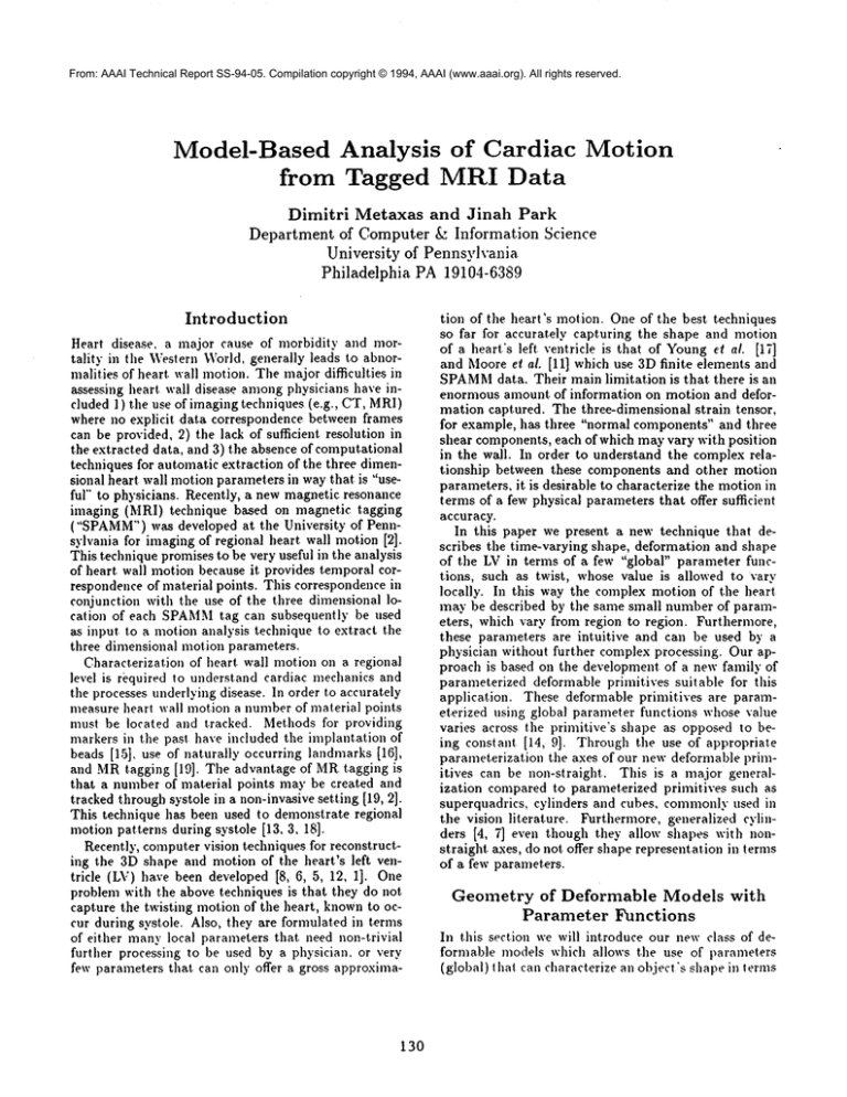
Figs. l(a-b) show a deformable model fitted
SPAMM
data at the first and last frames (times t =
and t = 5) during systole. In the above two time frames
(end-diastole and end-systole). Figs. l(c-d) show views
of the fitted model from the apex, corresponding to
Figs. l(a-b). Wecan easily observe the contracting motion as well as the twisting motion of the model.
In the following figure Fig. 2 we plot the extracted
model parameter functions over the 5 time frames.
Figs. 2(a-c) show plots of the model’s parameter functions al(u).a2(u) and a3(//), defining its length in the
x,y and z directions respectively.
For each frame we
plot. the ratio of each parameter function during frame
t = 2...5. with respect to its value at the initial frame
(t = 1). Fig. 2(d) shows plots of the model’s twisting
angle computed using the twisting parameter fimction
q (.u) and equation (i 1 ). In the interest of space we
not include plots of the bending parameter fimctions.
In all graphs. U = 0 corresponds to u,,,i, of the model
(the apex of the LV), and U = 12 corresponds to u,,m~
of the model (the base of the LV).
From these graphs, we can quanti~" the motion and
shape changes of the LV through time. For example, by
studying the graphs of al.o2 and a3 (Fig. 2(a-c)).
[5] L. D. Cohen and I. Cohen. "A Finite Element Method
Applied to New Active Contour Models and 3D Reconstruction
from Cross Sections", Proc. 2nd ICCV,
pp. 587-591, Japan 1990.
Meshes
[6] W-C. Huang and D. Goldgof. Adaptive-Size
for Rigid and Nonrigid Shape Analysis and Synthesis.
IEEE Transactions on Pattern Analysis, 15(6), pp. 611616, 1993.
"Representation
and
[7] D. Marr and K. Nishihara.
Recognition of the Spatial Organization of ThreeDimensional Shapes", Proc. Royal Society London B,
1978.
T.
Mclnerney and D. Terzopoulos. "A Finite Element
[8]
Model for 3D Shape Reconstruction and Nonrigid Motion Tracking", Proc. 4th International Conference on
Computer Vision, pp. 518-523, Berlin, Germany, 1993.
(a)
~"
ilnw;
............... ~..................... , .......... l~mC.q
_.
............
~oo ...........
o.o,~
:~;:.’ .........
I
¯r-- :- ~,~"
~- .......
t,’1"~.°.
....
.......
_." ,I :2
. ......... ~,. ]
.15.00
~.~)
I
I0o0
tl
as func-
[12] A. Pentland and B. Horowitz. "Recovery of Nonrigid
Motion and Structure"¯
IEEE Pattern Analysis and
Machine Intelligence, 13(7), pp. 730-742. July 1991.
[13] Rogers W, Shapiro E. Weiss J. Buchaiter M, Rademakers F, Weisfeldt M, Zerhouni E, "Quantification of and
correction for left ventricular systolic long-axis shortening by magnetic resonance tissue tagging and slice
isolation,’ ’ Circulation, 84, pp. 721-731, 1991.
[14] D.Terzopoulos and D. Metaxas. Dynamic 3D Models
with Local and Global Deformations: Deformable Superquadrics. IEEE Trans. Pattern Analysis and :llachine b, telligence, 13(7):703-714, 1991.
[15] Waldman LK, Fung YC, Covell JW., "Transmural myocardial deformation in the canine left ventrical: Normal in vivo three-dimensional finite strains," Circ Res.
57, pp. 152-163, 1985.
[16] Young, A.A., Hunter, P.J., Smaill. B.H., "Estimatiou of
epicardial strain using the motions of coronary bifurcations in biplane cineangiography," IEEE Trans Biomed
Eng, 39, pp. 526-531, 1992.
m conclude that the contraction
along z and V axes
. the apex of the LV is uniform and its magnitude of
retraction
during systole is approximately 20%. But
. the base of the LV, the contraction along y axis (beg approximately 10%) is less then one along x axis
,eing approximately 20%) making the base look more
liptical.
This result supports clinical study findings
here more stress is exerted at the apex during the LV
otion, and also there is an increased closeness to an
lipse of the LV base shape during systole.
Contrac~n along the z axis during systole is also quantified to
)proximately 20%.
References
l] A. Amlni and J. Duncan. "Pointwise tracking of LeftVentricular Motion in 3D," Proc. IEEE Workshop on
Visual Motion, pp. 294-298, Princeton, N J, 1991.
[17] Young. A.A., Axel L., "Three-dimensional Motion and
Deformation of the Heart V~rall"Radiology. 185. pp.
241-247, 1992.
[18] Young, A.A., lmai, H., Chang, C-N.. Axel. L.. "’Twodimensional LV deformation during systole." ("irculation in press, 1994.
[19] Zerhouni. E.A.. Parish. D.M., Rogers. W.J.. Yang. A..
Shapiro, E.P., "Human heart: Tagging with MRimaging - a method for noninvasive assessment of myocardial
motion," Radiology 169 pp. 59-63, 1988.
2] Axel, L.. Dougherty, L., "Heartwall motion: Improved
method of spatial modulation of magnetization for MR
imaging." Radiology, 17~, pp. 349-350, 1989.
i] Axel,
heart
tional
netic
1992.
[10] D. Metaxas and E. Koh, "Flexible Multibody Dynamics and Adaptive Finite Element Techniques for Model
Synthesis and Estimation," Proc. Second U.S. National
Congress on Computational Mechanics, Washington,
D.C., August, 1993.
[11] Moore, C., O’Dell, W., McVeigh, E., Zerhouni,
E., "Calculation of three-dimensiona~ left ventricular
strains form biplanar tagged MRimages," J Mug Res
Imag, 2, pp. 165-175, 1992.
(d)
igure 2: Some extracted
model parameters
ons of u for the first normal heart.
[9] D. Metaxas and D. Terzopoulos. Shape and Nonrigid
Motion Estimation Through Physics-Based Synthesis.
IEEE Trans. Pattern Analysis and ,Machine Intelligence, 15(6), pp. 569-579 , June, 1993.
L., Goncalves, R., Bloomgarden, D., "Regional
wall motion: Two-dimensional analysis and funcimaging of regional heart wall motion with magresonance imaging," Radiology, 183, pp. 745-750,
t] T. Binford. "Visual Perception by Computer", IEEE
Conference on Systems and Control, Dec. 1971.
133