Instance-Based Classifiers Dealing with Ambiguous Attributes and Class Labels
Hans Holland,
Miroslav Kubat
Jan Žižka
hholland@miami.edu, mkubat@miami.edu
zizka@iba.muni.cz
Department of Electrical and Computer Engineering
Institute of Biostatistics and Analyses
University of Miami
Masaryk University
Coral Gables, FL 33146, USA
Kamenice 126/3, 625 00 Brno, Czech Republic
Abstract
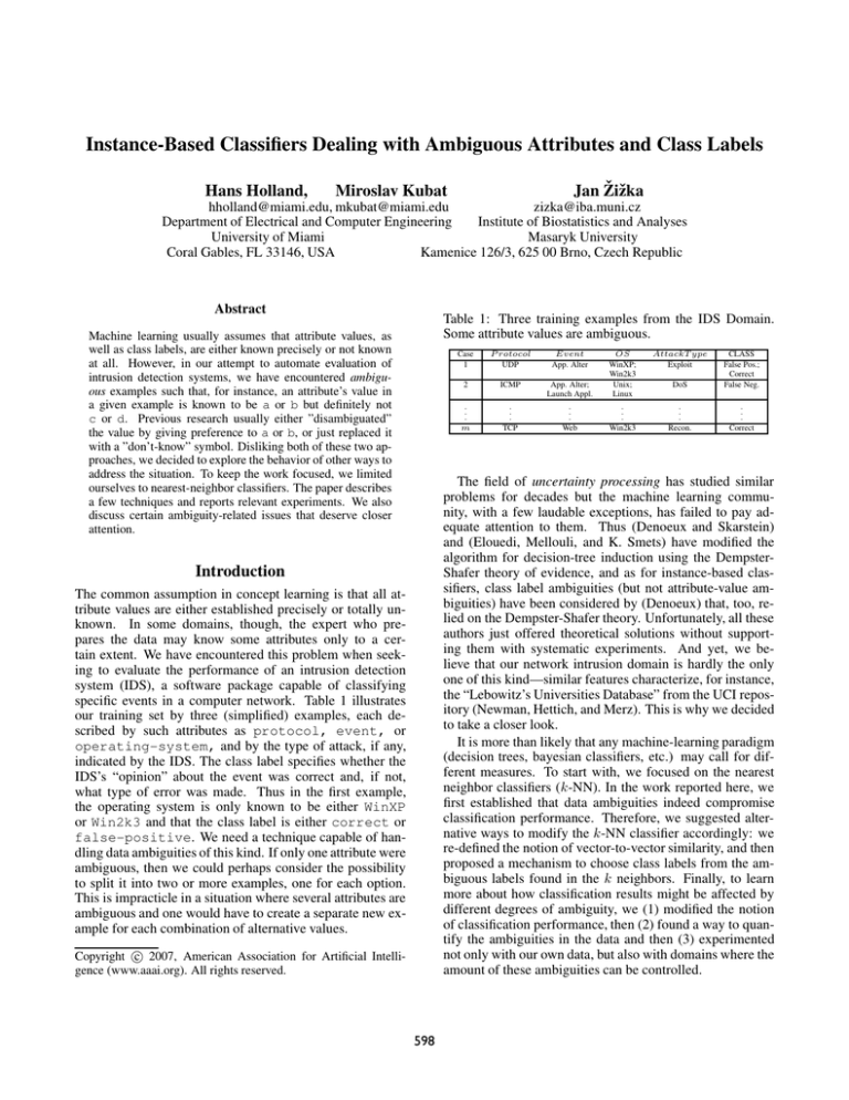
Table 1: Three training examples from the IDS Domain.
Some attribute values are ambiguous.
Machine learning usually assumes that attribute values, as
well as class labels, are either known precisely or not known
at all. However, in our attempt to automate evaluation of
intrusion detection systems, we have encountered ambiguous examples such that, for instance, an attribute’s value in
a given example is known to be a or b but definitely not
c or d. Previous research usually either ”disambiguated”
the value by giving preference to a or b, or just replaced it
with a ”don’t-know” symbol. Disliking both of these two approaches, we decided to explore the behavior of other ways to
address the situation. To keep the work focused, we limited
ourselves to nearest-neighbor classifiers. The paper describes
a few techniques and reports relevant experiments. We also
discuss certain ambiguity-related issues that deserve closer
attention.
Case
1
P rotocol
UDP
Event
App. Alter
AttackT ype
Exploit
App. Alter;
Launch Appl.
OS
WinXP;
Win2k3
Unix;
Linux
DoS
CLASS
False Pos.;
Correct
False Neg.
2
ICMP
.
.
.
m
.
.
.
TCP
.
.
.
Web
.
.
.
Win2k3
.
.
.
Recon.
.
.
.
Correct
The field of uncertainty processing has studied similar
problems for decades but the machine learning community, with a few laudable exceptions, has failed to pay adequate attention to them. Thus (Denoeux and Skarstein)
and (Elouedi, Mellouli, and K. Smets) have modified the
algorithm for decision-tree induction using the DempsterShafer theory of evidence, and as for instance-based classifiers, class label ambiguities (but not attribute-value ambiguities) have been considered by (Denoeux) that, too, relied on the Dempster-Shafer theory. Unfortunately, all these
authors just offered theoretical solutions without supporting them with systematic experiments. And yet, we believe that our network intrusion domain is hardly the only
one of this kind—similar features characterize, for instance,
the “Lebowitz’s Universities Database” from the UCI repository (Newman, Hettich, and Merz). This is why we decided
to take a closer look.
It is more than likely that any machine-learning paradigm
(decision trees, bayesian classifiers, etc.) may call for different measures. To start with, we focused on the nearest
neighbor classifiers (k-NN). In the work reported here, we
first established that data ambiguities indeed compromise
classification performance. Therefore, we suggested alternative ways to modify the k-NN classifier accordingly: we
re-defined the notion of vector-to-vector similarity, and then
proposed a mechanism to choose class labels from the ambiguous labels found in the k neighbors. Finally, to learn
more about how classification results might be affected by
different degrees of ambiguity, we (1) modified the notion
of classification performance, then (2) found a way to quantify the ambiguities in the data and then (3) experimented
not only with our own data, but also with domains where the
amount of these ambiguities can be controlled.
Introduction
The common assumption in concept learning is that all attribute values are either established precisely or totally unknown. In some domains, though, the expert who prepares the data may know some attributes only to a certain extent. We have encountered this problem when seeking to evaluate the performance of an intrusion detection
system (IDS), a software package capable of classifying
specific events in a computer network. Table 1 illustrates
our training set by three (simplified) examples, each described by such attributes as protocol, event, or
operating-system, and by the type of attack, if any,
indicated by the IDS. The class label specifies whether the
IDS’s “opinion” about the event was correct and, if not,
what type of error was made. Thus in the first example,
the operating system is only known to be either WinXP
or Win2k3 and that the class label is either correct or
false-positive. We need a technique capable of handling data ambiguities of this kind. If only one attribute were
ambiguous, then we could perhaps consider the possibility
to split it into two or more examples, one for each option.
This is impracticle in a situation where several attributes are
ambiguous and one would have to create a separate new example for each combination of alternative values.
c 2007, American Association for Artificial IntelliCopyright gence (www.aaai.org). All rights reserved.
598
Problem Statement
Table 2: Ambiguous class labels from a k-NN classifier
The learner’s input consists of training examples, [x, C(x)],
such that x = (x1 , x2 , . . . , xM ) describes the example by
discrete attributes and C(x) is the class label. We assume
that any attribute, and any class label, can be ambiguous—
for instance, xi = [a, b] is interpreted as meaning that the
value of xi is either a or b (but no other value). The task
is to induce a classifier that will determine the class labels
of future examples. When evaluating its performance, we
have to keep in mind that the testing examples, too, can be
ambiguously described. This has to be reflected in the employed performance criterion—if a testing example’s class
is known to be either C1 or C2 , then a classifier that predicts
C1 should be deemed less accurate than one that predicts
[C1 , C2 ].
Let N be the number of testing examples, let Ci,known
be the set of class labels of the i-th testing example, and let
Ci,classif be the set of class labels given to the i-th testing
example by the classifier. We evaluate the classification performance of this classifier by the following formula:
N
1 Acci ;
where
N i=1
|Ci,known Ci,classif |
Acci =
|Ci,known Ci,classif |
AmbA =
Class Labels
Nearest Neighbor 1
Nearest Neighbor 2
Nearest Neighbor 3
Table 3: Voting about the class label based on the nearest
neighbors listed in Table 2
Wf actor (C)
C1 = 13 12
C2 = 13 12
C3 = 13 02
C4 = 13 02
nA − 1
nT − 1
(1)
(2)
Wf actor (c) =
(3)
k
1 Ni,c
k i=1 Ni,total
(5)
For the case of the three nearest neighbors from Table 2,
the class weights are calculated in Table 3. The system
chooses classes whose weights exceed a user’s threshold, θ.
For instance, if θ = 0.4, class C2 is chosen; if θ = 0.2,
classes [C1 , C2 ] are chosen.
Example-to-Example Similarity
Suppose that x = (x1 , . . . xM ) and y = (y1 , . . . yM ) are
examples. Nearest-neighbor classifiers usually calculate the
similarity of these x and y from the similarity along the individual attributes:
m
1 nA(j) − 1
× 100%
m j nT (j) − 1
+ 01 ⇒ 0.278
+ 11 ⇒ 0.500
+ 01 ⇒ 0.111
+ 01 ⇒ 0.111
1
3
0
3
1
3
1
3
In the example from Table 2, the 3-NN classifier has already
identified the three nearest neighbors, some of which have
more than one class label (because the true class is known
only partially). Labeling the testing example with a union of
these labels would not reflect the different degree of “focus”
in the individual neighbors. Thus the fact that the first neighbor suggests classes [C1 , C2 ] and the third neighbor suggests
only C2 seems to indicate we should have more confidence
in the latter.
This is why we weigh each label by the focus of the given
example. Let Ni,c = 1 if class c is found among the labels
of the i-th nearest neighbor and let Ni,c = 0 if it is not.
If Ni,total is the number of labels in the i-th nearest neighbor, then, for k nearest neighbors, we calculate the weight
of class c as follows:
This ensures that AAmb = 0 if the value is known precisely (nA − 1 = 0) and AAmb = 1 if the value is totally unknown. Note that each attribute must be able to acquire at least two different values so that nT > 1. The total
amount of attribute-value ambiguity in the data can be assessed either by taking the average value of AAmb over all
example-attribute pairs or over only those example-attribute
pairs where the attribute value is ambiguous. In the following formula, m is the number of example-attribute pairs considered.
AAmbtotal =
+
+
+
+
Voting Mechanism
Furthermore, we need a mechanism to quantify the
amount of ambiguity in the data. Suppose that, in a given example, an attribute is given nA out of nT of different values.
For instance, if the attribute can acquire values [a, b, c, d, e]
and is known to be either a or b, for the given example, then
nT = 5 and nA = 2. The amount of ambiguity is then
quantified as follows:
AAmb =
C1 or C2
C1 or C3 or C4
C2
(4)
S(x, y) =
n
s(xi , yi )
(6)
i=1
Handling Ambiguity in k-NN Classifiers
In our context, s(xi , yi ) has to reflect the ambiguities in
xi and yi . Let us show three simple ways on how to handle
the problem in traditional k-NN classifiers, and then proceed
to our own solution.
Let us first discuss how to handle the voting mechanism,
and then turn our attention to the assessment of example-toexample similarity.
599
Traditional Nearest Neighbor Approaches. Classical
k-NN classifiers usually assume that each attribute is either
known precisely or totally unknown (replaced with a question mark). In our experiments, we used the following three
alternatives.
Table 4: Two ambiguous examples
Example x
x1 SUMMER or SPRING
HUMID
x2
DAY
x3
k-NNa: If xi = yi , then s(xi , yi ) = 0; if xi = yi , then
s(xi , yi ) = 1; and if a question mark is encountered in either
xi or yi , then s(xi , yi ) = 1. These values are then summed
over all M attributes:
S(x, y) =
s(xi , yi ) =
M
s(xi , yi );
where
|SP RIN G|
||
|SP RIN G,SUMMER| + |DRY,HUMID|
|
+ |DAY
|DAY |
= 12 + 02 + 11 = 1.5
S(x, y)kAmbN N =
(7)
i=1
1
0
1
yi =
xi
yi = xi
yi = ? or xi = ?
Fuzzy Nearest Neighbor: k-fuzzyNN
For the sake of comparison with some earlier work in uncertainty processing, we also implemented a fuzzy voting
mechanism. The idea is to consider the degree of membership of the training example in a class. We use the following
definitions:
(8)
k-NNb: If the ambiguities are rare, we can afford ignoring
the unknown attribute values altogether. For all the remaining attributes, xi = yi implies s(xi , yi ) = 0 and xi = yi
implies s(xi , yi ) = 1. Denoting by M 1 the number of unambiguous attributes, we use the following formula:
S(x, y) =
M1
i=1
• nc . . . number of classes,
• k . . . number of nearest neighbors,
• 1 ≤ j ≤ k . . . j-th neighbor,
s(xi , yi );
s(xi , yi ) =
1
0
where
(9)
xi
yi =
yi = xi
(10)
• μi (yj ) . . . membership of the neighbor, yj , in the i-th
class,
• μi (x) . . . membership of the training example, x, in the
i-th class,
• x − yj . . . the distance between x and yj
k-NNc: Yet another possibility is to replace each question
mark with the most frequent value of the given attribute. The
similarity-calculating formula then remains unchanged:
S(x, y) =
M
i=1
s(xi , yi ) =
Example y
y1 SPRING
DRY
y2
DAY
y3
s(xi , yi );
1
0
where
xi
yi =
yi = xi
• 1.0 ≤ w ≤ 2.0 . . . a fuzzy parameter
The following formula, based on ideas developed by
(Keller), represents the normalized membership for each of
the class labels.
(11)
k
−
2
μi (yj ) · (x − yj w−1 )
, i = 1, 2, . . . , nc
μi (x) =
2
k
− w−1
)
k=1 (x − yj (14)
Note that we are using distance x − yj instead of similarity. Furthermore, note that the formula involves two parameters: w and θf uzzy , the latter being a threshold that controls the class selection.
j=1
(12)
Ambiguous Nearest Neighbor Approach: k-AmbNN.
More complicated is the case where the training set gives,
for the given example-attribute pair, a proper subset of possible values. Let us denote by xi and yi the sets of values of
the i-th attribute in x and y. To make sure that the similarity
between x and y reflects the relation between the sets xi and
yi , we use the following formula.
n
|xi yi |
S(x, y)kAmbN N =
(13)
|xi yi |
i=1
Experimental Data
Primarily, we wanted to apply our algorithms to the domain
that has inspired this research—intrusion detection. Then,
to learn more about the behavior of the individual formulas,
we also used one domain from the UCI repository and one
synthetic domain.
Note that the formula degenerates into the “traditional”
approach where at least one of the values is replaced with a
“?” (see above).
For illustration, consider a simple domain where the examples are described by season (SPRING, SUMMER,
FALL, WINTER) air quality (DRY, HUMID), and
day-time (DAY, NIGHT). The similarity of the two examples from Table 4 is obtained as follows:
Network Intrusion Detection System Data
The data file was compiled from observations made on a
concrete computer network as a result of a number of measurements. The collected data included the protocol of the
incoming network request, the event that took place due to
the request, analyzed attack type, type of operating system
600
AT1
Table 5: Illustration of IDS Data Definition (abridged and
simplified
P rotocol
UDP
TCP
ICMP
Event
Web
App. Alter
Launch
App.
Install
Term.
Key Proc.
Auto
Launch
AttackT ype
Recon.
Exploit
DoS
OS
Linux
Unix
WinXP
System
NIDS
SIV
LM
x
z
y
Class
False Pos.
False Neg.
Correct
AT2
n
AT6
c2
Win 98/Me
Win2k
c
c4
Win2k3
AT3
o,m
d
e
c1
a
b
s
c1
c3
c1
c3
AT4
t,r
AT5
p
q
c2
c4
Figure 1: The decision tree is used to create a synthetic domain initially.
targeted in the attack, system used for intrusion detection,
and possible classification labels: False Positive, False Negative, and Correctly classified.1
Table 5 summarizes attributes that acquire ambiguous values. The ambiguity is due to the network administrator’s
limited ability to interpret the corresponding log files. Other
attributes were unambiguous—in reality, there were 10 attributes and 126 examples. The amount of ambiguity according to Equation 4 is 30%.
AT1
x
z
y
AT2
n
c2
UCI Domain
c4, c2, c1
AT3
o,m
a
b
c4, c3, c1
c1
c3
Figure 2: The decision tree is used to re-classify the data for
purposes of introducing ambiguous class labels.
The Lebowitz’s universities domain was compiled
in July 1988 and consists of 285 instances (including duplicates) with 17 attributes.
One of the attributes (academic-emphasis) acquires ambiguous values, other attributes have missing values. We eliminated duplicate examples.
labeling more ambiguous than necessary. We measured the
classification performance by the AAmb metric defined by
Equation 1. For the synthetic data, Table 6 shows the values
of AAmb for different values of θ. The results indicate that
the optimum cut-off is somewhere between 0.3 and 0.5, and
that its optimum value depends also on the number, k, of the
nearest neighbors employed.
In the experiments reported in the rest of this section,
we always used θ = 0.3 while understanding that the finetuning of θ to the specific needs of a concrete domain might
further improve the results. Further on, the reader is reminded that, for ambiguous domains, we have defined a performance metric, AAmb, whose behavior is different from
the classical classification accuracy. If a testing example
belongs to classes (C1 , C2 ) and the classifier outputs (C2 ),
then Acc = 0.5. Note that the values of AmbA are typically
lower than those of the classification accuracy.
For the fuzzy nearest neighbor approach (k-fuzzyNN), established (by experiments not reported here) that the best
choice of the parameter w was—at least for the domains we
worked with—w = 2.0.
Figure 3 compares the performance of k-AmbNN with
Synthetic Domains
Maximum experimental flexibility is provided only by synthetic domains that allow the researcher freely to adjust data
parameters. The one we used in this research was created
with the help of decision trees. First, we randomly generated artificial examples described by 10 multi-valued discrete attributes. Then, we manually created the decision tree
shown in Figure 1 and truncated it, obtaining the tree in Figure 2 that was then used to classify the data. Note that some
of the leaves contain more than one class—this introduces
the class-label ambiguity. Attribute ambiguity is introduced
by randomly selecting an attribute and adding the most frequently occurring value to it. The amount of ambiguity is
controlled by the parameter AAmb defined earlier—in alternative versions of the data, AAmb ranged from 10% to 50%.
Experimental Results
First, we wanted to learn how the performance is affected
by the cut-off point, θ, used in the voting mechanism—
recall that the testing example is assigned all class labels for
which Wf actor (c) > θ. High values of θ lead to the “crisp”
single-label case, or even to the situation where no class label exceeds θ. Conversely, very low values will render the
Table 6: AmbA-performance for different cut-off points and
k-values as evaluated on synthetic domain with AAmb =
30%.
cut-off
k=1
k=3
k=5
k=9
1
Sample
domains
can
be
downloaded
from
http://umsis.miami.edu/˜hholland/k-ANN/.
For additional support, please contact Hans Holland (hholland@miami.edu)
601
0.1
0.385
0.285
0.149
0.037
0.2
0.385
0.285
0.459
0.267
0.3
0.385
0.366
0.459
0.466
0.4
0.385
0.366
0.416
0.503
0.5
0.385
0.366
0.416
0.398
0.6
0
0.112
0.248
0.286
0.7
0
0.112
0.019
0.019
0.8
0
0
0.019
0.019
University Domain
Network Intrusion Detection System Domain
1
1
k−AmbNN
k−NN
k−NNfuzzy
0.8
0.8
0.7
0.7
0.6
0.5
0.4
0.6
0.5
0.4
0.3
0.3
0.2
0.2
0.1
0.1
0
0
0
1
2
3
4
5
6
7
Number of selected neighbors (k)
8
9
k−AmbNN
k−NN
k−fuzzyNN
0.9
Ambiguous Accuracy (AmbA)
Ambiguous Accuracy (AmbA)
0.9
10
0
1
2
3
4
5
6
7
Number of selected neighbors (k)
8
9
10
11
Figure 3: Comparing the performance of k-AmbNN with
that of k-NN on the IDS domain.
Figure 4: Comparing the performance of k-AmbNN with
that of k-NN on the university Domain.
that of k-NN and k-fuzzyNN in the intrusion detection domain for different values of k. To be able to use k-NN,
we replaced ambiguous values with question marks. The
individual points in the charts have been obtained as averages from the 5x2 cross-validation, a methodology recommended for the assessment of machine learning algorithms
by (Dietterich). The reader can see that k-AmbNN consistently outperforms the other approaches over a whole range
of k-values. Since k-NN systematically underperforms kAmbNN, we conclude that replacing partial ambiguity with
total ambiguity is indeed unnecessary and harmful. Interestingly, whereas k-NN’s performance dropped with the growing value of k (perhaps due to the sparseness of the data),
k-AmbNN’s performance grew with increasing k. The margin between k-NN and k-AmbNN is statistically significant
according to the two-tailed t-test with a confidence level of
2%. The fuzzy approach does not seem to be appropriate,
here. We surmise that our ambiguities are too simple for the
fuzzy-set approach to fully unfold its strength.
Figure 4 corroborates all these observations by experiments with the university domain. In this sparser, but
less noisy domain, even k-AmbNN’s performance tended to
drop with growing k, although even here we seem to have a
reason (at least for small k) to claim that k-AmbNN is more
robust regarding the increasing values of k. We cautiously
suggest that the experiments with the first two domains indicate that k-AmbNN offers not only higher performance, but
also higher robustness with respect to k. Note that, somewhat surprisingly, the fuzzy approach again does not show
its strength.
In the remaining experiments, we modified our system so
that it automatically chooses the optimum k value. This is
achieved by an “induction” algorithm that estimates the classification accuracy (applying the 5-fold cross-validation approach to the training set) for different values of k and then
selects the one that promises the highest performance. The
same approach could in principle have been employed also
for the choice of the θ-threshold used in the voting scheme
but we used the fixed θ = 0.3 not to complicate things.
Figure 5 shows how the classification performance depended on the amount of ambiguities in the data. While
k-fuzzyNN and k-NN appear relatively unperturbed by this
parameter, k-AmbNN’s performance drops conspicuously
with growing values of AAmb. The observation leads us to
assume that k-AmbNN is more appropriate where the domain ambiguity is limited.
Conclusion
Having surmised that classical nearest neighbor classifiers
may be inadequate to deal with ambiguously described
examples, we proposed our own modification, k-AmbNN
(ambiguous nearest neighbor), and compared its performance with that of the classical k-NN rule and with that of
a solution suggested by the fuzzy-sets community.
Importantly, we have realized that ambiguous domains
call for a specially designed performance metric. Our experiments with three different domains indicate that the performance of the k-AmbNN compares very favorably with
the performance of modest modifications of the classical kNN classifier and with k-fuzzyNN. While k-NN apparently
suffers from the replacement of partial ambiguity with the
”don’t know” symbol, k-fuzzyNN seems to have been meant
for more sophisticated uncertainties than those encountered
in our domains.
The reader may complain that the paper fails to report experiments with an impressive array of benchmark domains
as is common in the machine-learning literature. The truth is
that we found in the UCI repository only one such domain,
university. We speculate that other UCI domains might
originally have contained ambiguities, too, but their authors
sanitized them because the community was only used to totally unknown attribute values. However, the experience re-
602
as for the experimental data we have used, please contact
Hans Holland—hholland@miami.edu.
Synthetic Decision Tree Domain
1
k−AmbNN
k−NN
k−NNfuzzy
0.9
Acknowledgment
Ambiguous Accuracy (AmbA)
0.8
The research was partly supported by the NSF grant
IIS-0513702.
0.7
0.6
0.5
References
0.4
Bezdek, J.C. (1981). Pattern Recognition with Fuzzy Objective
Function Algoritms, Plenum Press, New York
Dietterich, T. G. (1998). Approximate Statistical Tests for Comparing Supervised Classification Learning Algorithms. Neural
Computation, 10, (7) pp. 1895–1924.
Denoeux, T. (1995). The k-Nearest Neighbor Classification Rule
Based on Dempster-Shafer Theory. IEEE Transactions on Systems, Man, and Cybernetics, Vol.25, pp. 804–813
Denoeux, T. and Skarstein, M. (2000). Induction of Decision
Trees from Partially Classified Data Using Belief Functions, Proceedings of SMC pp. 2923–2928
Dunn, J.C. (1973). A Fuzzy Relative of the ISODATA Process and
Its Use in Detecting Compact Well-Separated Clusters, Journal of
Cybernetics 3: pp. 32–57
Elouedi, Z. Mellouli, and K. Smets, P. (2001). Belief Decision
Trees: Theoretical Foundations International Journal of Approximate Reasoning Vol.28, pp. 91–124
Keller, J. M., Gray, M. R, and Givens, J. A. (1985) A Fuzzy
k-Nearest Neighbor Algorithm. IEEE Transactions on Systems,
Man and Cybernetics, 15(4), pp. 80–85.
Newman, D.J., Hettich, S., Blake, C.L. and Merz, C.J.
(1998). UCI Repository of Machine Learning Databases
[http://www.ics.uci.edu/ mlearn/MLRepository.html]. Irvine,
CA: University of California, Department of Information and
Computer Science.
Shafer, Glen (1997). A Mathematical Theory of Evidence, Princeton University Press
Shafer, G., and Pearl, J. (eds.) (1990). Readings in Uncertain Reasoning. Morgan Kaufmann.
Vannoorenberghe, P. (2004). On Aggregating Belief Decision
Trees Information Fusion, Vol. 5, pp. 179–188
Vannoorenberghe, P. & Denoeux, T (2002). Handling Uncertain Labels in Multiclass Problems Using Belief Decision
Trees.Proceedings of IPMU’2002, Anneey, France, pp. 1919–
1926
0.3
0.2
0.1
0
0
10
20
30
40
Amount of Ambiguity introduced into the data set (AAmb)
50
60
Figure 5: Comparison of the performance of k-AmbNN, kNN, k-fuzzyNN on the decision-tree-generated synthetic domains, as measured for different degrees of ambiguity.
ported in this paper indicates that the fact that, say, season is
either spring or summer—but not fall or winter—is
qualitatively different from the “question-mark” situation.
Finally, our work suggests there is a need to search for
better methods to quantify such aspects as the degree of data
ambiguity. To this end, we have proposed our own formula
but we hope that other researchers will scrutinize its shortcomings and limitations, and, if necessary, develop more appropriate methods. The same applies to the formula we have
used to assess the classification performance.
This brings us to suggestions for further research. In an
attempt to make the paper self-contained, and to avoid advanced theoretical paradigms that might obscure the simple ideas and observations we wanted to share, we labored
hard to make our solution as simple as possible. However, more sophisticated approaches can be employed even
in the unassuming paradigm of nearest-neighbor classifiers.
For instance, the fuzzy-set theory (Bezdek) certainly offers
many more possibilities than the one from (Keller). Also
the voting mechanism could have relied on sounder theoretical principles such as those developed in the frame of the
Dempster-Shafer theory. For an early attempt to employ this
paradigm in domains with ambiguous class labels (but not
attribute values), see (Denoeux).
Finally, we would like to encourage work in other fields
of machine-learning. In the realm of decision trees, the
pioneering research reported by (Vannoorenberghe; Vannoorenberghe and Denoeux) has suggested theoretical solutions that still wait for systematic experimental evaluation. We are sure that other frameworks—such as linear
classifiers, Bayesian classifiers, neural networks, or support
vector machines—offer a rich source of opportunities that,
lamentably, no one has yet attempted to explore. Our paper
hopes, in its modest way, to help change this situation.
For the code of the algorithms used in this paper, as well
603