Shape Depth
ECARES & Département de Mathématique, Université Libre de Bruxelles
G. VAN BEVER*, D. PAINDAVEINE, gvbever@ulb.ac.be
1. Tukey’s halfspace depth and Mizera’s tangent depth.
In the multivariate location setup, Tukey (1975)
Mizera (2002) generalized the concept of depth
introduced the notion of halfspace median as
to any parametric model. Given a C 1 objective
argmaxµ∈IRpHD(µ; FX), the vector with max-
function F : Θ×X → IR, he defined the tangent
imum halfspace depth. Here,
depth of θ̃ ∈ Θ as
T D θ̃, FX = HD 0p; ∇θ F (θ̃, X) .
0
HD(µ; FX) = infp−1 IPFX {u (X − µ) ≥ 0} .
u∈S
In the empirical setup, the halfspace depth of µ can be seen as the smallest
number of observations one may remove before µ lies outside the convex hull
of the remaining data.
With respect to the construction of the maximum likelihood estimator, he
suggested F (θ, X) = log fθ (X) as a candidate for the objective function.
2. The shape parameter.
In many classic multivariate problems, it is sufficient to know
a normalized version of the dispersion/scatter matrix in order
to perform the analysis (PCA, CCA, test of sphericity, etc.)
The scale parameter associated with Σ is σS2 = S(Σ). The shape parameter
is VS = Σ/S(Σ). Denote
S
Vp
= {V ∈ Sp |S(V) = 1}. Classical choices of
1/p
scale functionals are SO (Σ) = Σ11, ST (Σ) = tr(Σ)/p and SD (Σ) = |Σ|
.
We are interested in the shape parameter of p-variate elliptical distributions,
Definition
+
IR0
A scale functional is a (i) 1-homogeneous function S : Sp →
(i.e.
∂S
S(λΣ) = λS(Σ)) such that (ii) S is differentiable, with ∂Σ11 (Σ) 6= 0 for
all Σ ∈ Sp and (iii) satisfies S(Ip) = 1.
with general density
cp,g1
c̃p,g
(d(x,
x 7→
g
θ;
Σ))
=
g
(d(x,
θ;
V
))
=
f
(x),
1
S
θ,V,g
1/2
1/2
|Σ|
|VS |
1/2
−1
0
where d(x, θ; Σ) = (x − θ) Σ (x − θ)
, Σ ∈ Sp.
3. Shape depth.
Hallin and Paindaveine (2006) showed that the score is given by
d d
0
V
⊗2 −1/2
∇VF (V, X) ∝ MS V
vec ϕg1( ) UU − Ip ,
σS σS
−1/2
0
V
MS
(X − θ)/d and ϕg = −g /g.
is the
V 0
˚
(p(p+1)/2−1)×p matrix such that (M ) (vech)(v)
= vec(v) for all matrix
with d = d(X, θ; V), U = V
S
0
v ∈ Sp such that (∇S(vech(V)) (vech(v)) = 0. The unspecification of scale
2
σS
leads to rather consider the efficient scores (obtained from projections along
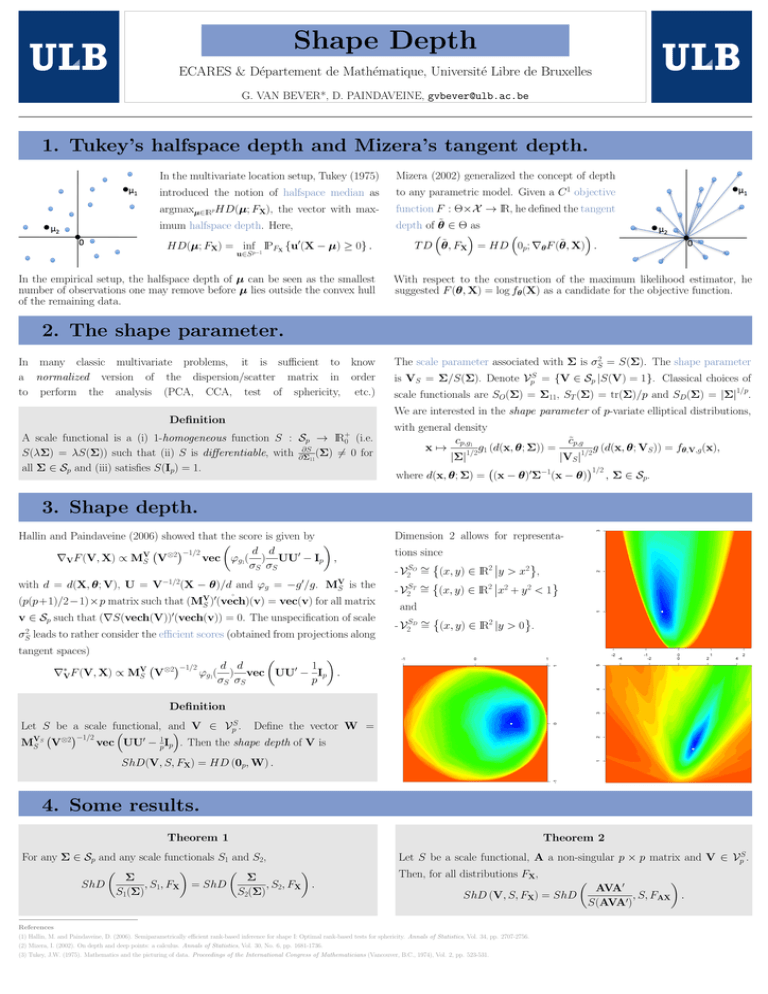
Dimension 2 allows for representations since
SO ∼
2
- V2 = (x, y) ∈ IR y > x2 ,
ST ∼
2 2
- V2 = (x, y) ∈ IR x + y 2 < 1
and
SD
- V2
2
∼
= (x, y) ∈ IR |y > 0 .
tangent spaces)
∗
∇VF (V, X)
∝
V
MS
V
⊗2 −1/2
1
d d
0
ϕg1( ) vec UU − Ip .
σS σS
p
Definition
S
Let S be a scale functional,
and
V
∈
V
.
Define
the
vector
W
=
p
VS
⊗2 −1/2
MS V
vec UU0 − p1 Ip . Then the shape depth of V is
ShD(V, S, FX) = HD (0p, W) .
4. Some results.
Theorem 1
For any Σ ∈ Sp and any scale functionals S1 and S2,
Σ
Σ
, S1, FX = ShD
, S2, FX .
ShD
S1(Σ)
S2(Σ)
Theorem 2
Let S be a scale functional, A a non-singular p × p matrix and V ∈
Then, for all distributions FX,
0
AVA
ShD (V, S, FX) = ShD
, S, FAX .
0
S(AVA )
References
(1) Hallin, M. and Paindaveine, D. (2006). Semiparametrically efficient rank-based inference for shape I: Optimal rank-based tests for sphericity. Annals of Statistics, Vol. 34, pp. 2707-2756.
(2) Mizera, I. (2002). On depth and deep points: a calculus. Annals of Statistics, Vol. 30, No. 6, pp. 1681-1736.
(3) Tukey, J.W. (1975). Mathematics and the picturing of data. Proceedings of the International Congress of Mathematicians (Vancouver, B.C., 1974), Vol. 2, pp. 523-531.
S
Vp .