From: AAAI Technical Report WS-98-07. Compilation copyright © 1998, AAAI (www.aaai.org). All rights reserved.
Modeling periodic
functions
for time series
analysis
Anish Biswas
Department of Mathematics and Computer Science
University of Tulsa
600 South College Avenue
Tulsa, OK 74014
E-mail: abiswas@euler.mcs.utulsa.edu
Abstract
Timeseries problemsinvolve analysis of periodic
functions for predicting the future. Aflexible regression method should be able to dynamically
select the appropriate modelto fit the available
data. In this paper, we present a function approximation schemethat can be used for modeling periodic functions using a series of orthogonal
polynomials, named Chebychev polynomials. In
our approach, we obtain an estimate of the error
due to neglecting higher order polynomials and
thus can flexibly select a polynomialmodelof the
proper order. Wealso showthat this approximation approachis stable in the presence of noise.
Keywords: Function approximation,Orthogonal
nomials
the model can be improved. Wehave also provided the
convergence proof of the algorithm, which says that under infinite sampling this method is guaranteed to give
accurate model and the level of accuracy is limited only
by error due to truncation of the series.
Chebychev
Chebychevpolynomials are a family of orthogonal polynomials (Geronimus 1961). Any function f(x) may
approximated by a weighted sum of these polynomial
functions with an appropriate selection of the coefficients.
OO
f(x)
poly-
Introduction
Analysis of time series data plays an important role
in finance and marketing. A model derived from past
data can help to predict future behavior of the phenomenon under study. For example , models predicting demand for product can be used to direct capital
allocation. For analysis of time series data, we, in general, start with a predetermined model and try to tune
its parameters to fit the data. For example, we may
choose to fit a linear model to the data. for a flexible approximation scheme, however, a model should be
chosen dynamically, based on data. In this paper, a
function approximation scheme is presented, which can
be used for modeling periodic functions. Wehave used
a series of orthogonal polynomials, called Chebychev
polynomials for approximating time series data. We
know that any function can be represented with an infinite series of Chebychevpolynomials. But we cannot
work with an infinite series and use only a finite number
of terms to derive an approximation. This method gives
an approximate model for the data using n Chebychev
polynomials where the number of polynomials can be
dynamically decided from the data. The approximated
model with n Chebychev polynomials gives the least
squared error with n polynomials.
Furthermore, our algorithm allows incremental development of the model, i.e. with each piece of data,
polynomials
a0
= -~ + E ai * 7](x)
i=1
where
and
2 F f(x) * 7](x)
ai=-zrJ_l
~-1---’-’~ dx.
Working with an infinite series is not feasible in
practice. Wecan, however, truncate the above series
and still obtain an approximation, ](x), of the function (Gerald & Wheatly 1992). The Chebychev polynomials converges faster than the Taylor series for the
same function (Gerald g: Wheatly 1992). Let us assume
we are using only the first n terms of the series. For a
rapidly converging series, the error due to truncation is
approximately given by the first term of the remainder,
i.e., a,~Tn(x). Wehave chosen Chebychev polynomials
for function approximation because truncation points
can be chosen to provide approximate error bounds.
It should be noted that the expansion of a function
f(x) with n Chebychev polynomials, gives the least
squared polynomial approximation with the n polynomials (Foxand & Parker 1968).
To produce a viable mechanism for building a model
based on Chebychev polynomials would require the development of an algorithm for calculating the polynomial coefficients. Wewould also need to prove that this
algorithmic updates would result in a convergence of
the approximated function to the actual time function
1.5
i
,
,
,
i
I
i
i
1.2
i
i
i
i
i
i
0.8
t.....................
~"
0.6
"
\
t
i,
,
)
ap~n~x(r(x))
abs(~ln(5*x))
i
1
0,5
o
)
/~
approx(r(x))
sin(lO*x)....
i ~
,
i L
i
i Z
i J
i
i
i
0.4
4).5
0.2
11
-1.5
-1
-0.8
-0.6
4).4
-I).2
(I,2
114
06
08
I
-0,8
Lll
I
-0,6
~,i/
I
-0.4
I
-ILl
~
i
O
X
t/
I
0.2
I
0,4
I "l
I},6
I
(ill
Figure 1: Approximating f(x) = sin(lO*x) for Number
of Chebychev Polynomials used = 20 and number of
data points = 1000.
Figure 2: Approximating f(x) = Isin(5*x)l for Number
of Chebychev Polynomials used = 10 and number of
data points = 1000.
underlying the sampled data. Weprovide such an algorithm and the associated convergence theorem in the
next section.
Approximations
of periodic
functions
Weknow that a periodic function S(x) can in general
be expressed as
An algorithm
to get the temporal
model
from time series
data
Let f(x) be the target function of x and f(x) be its
approximation based on the set of samples S = {Sj},
where Sj = (xj, v~:j)Vj = 1, 2,..., k and k = Numberof
instances and v~j = f(xj). Wemay have to change the
scale for the values x j, so that all the values are in the
range [-1 : 1]; then we get the approximated function
in the range [-1 : 1], which we may need to scale back
to get the desired value.
Let n be the number of Chebychev polynomials we
are going to use for the purpose of learning. Let
~(x) i E [0..n] be the Chebychev polynomials. The
steps of the algorithm are:
1. InitializeCi=0,
Vi=0,1,2,...,n
2. For all j do
3. Vi = 0,1,2,...,n
2x/l - x
4. End for
5. Set
n
Co + ~G*Ti
= s<, (-7i=l
where K = ¢(k) , is function of number of interactions.
Theorem 1 Under infinite
sampling the algorithm
can approximate the actual function.
Proof: See Appendix.
f(x) ---- f(x -t- T*
where T is the period and n E [0, 1,2,...] . So the nature of the function in a single period and the length
of the period is enough for the prediction of behavior
for unknown x values. From our approximation scheme
we get these two pieces of information and can successfully predict the behavior of the functional values for
unseen situations. Wehave taken some typical periodic
functions and tested the algorithm for those functions:
f(x) --- sin(x 10), an d f( x) -=Isi n(x * 5)1
Weknowthat the error due to truncation is given by the
first term in the series and thus we can flexibly decide
the number of terms to be chosen for approximation.
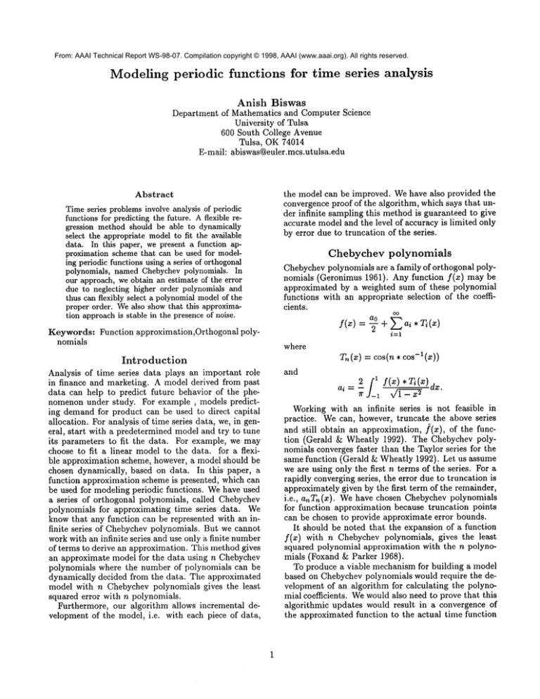
The actual functions and the polynomial approximations obtained for these two functions are presented in
Figures 1 and in Figures 2. Wehave given each data
point sequentially into the algorithm and the resulting
functions generated are found to be fairly good approximations of the underlying functions. Thus we can get a
good measure of the period and nature of the function
in a period. Wecan use this informations to get the
functioal values in unseen points.
Wehave also shown the nature of improvement of the
model with more data points for the f(x) Isin(x * 5)
in Figures 3. Wehave calculated error as the average
of the difference of approximate functional values and
the accurate values, over a set of sampled points in the
interval [-1 : 1]. It shows that the approximation accuracy increases rapidly with number of points.
Effects of Noise: Wehave also tested the approximation scheme under noisy data, where noise is added
0.3
0.4
0.35 1
0,25
0.3’-
No m)l~-~.d.,~).l
....
~.d.~O.3
.....
~.d.-05.....
Em)r --
~,
i;
0.25
~.j,,\
0,2
0,15
o.1
0.05
0,05
I
200
I
400
I
600
I
I
/
R00 I(X~ 1200
Numhc¢
of Data[xfints
I
1400
I
I
1604) 1800
4)
0
Figure 3: Nature of decreasing error in approximating
f(x) = Isin(x 5)] Number of Chebychev Pol ynomials
used is 11 and sampling resolution is 1000.
)
I(X)0 I
Number
ofdatll[~)inl~;
1404)
I(~10
I~.)
20{}0
Figure 4: Nature of decreasing error in approximating
f(x) = sin(x, 10) under noise Number of Chebychev
Polynomials used is 20 and sampling resolution is 1000.
of greater resolution is received. Wehave
to each data point. Here we assume that the random
noise follow a Normal distribution.
Wehave run experiments with random noise following Normal distribution(#
= 0,~) where g =
= 0.1, ~ = 0.3, g = 0.5 values are applied where
value of f(x) is in the range [-1 : 1]. Wehave investigated the nature of decreasing error with more
data points and see that the process is resilient to
noise as average error do not increase rapidly with
noise shownin Figures 4.
¢ ,fi
(/(x~)
~(x~)
--
where ¢ is a function of no of interactions
given by ¢ = 2" So,we get,
and can be
j=l
Now,in case of infinite
tion, we have,
Conclusion
Wehave presented an algorithm that can build a model
from the time series data where this model is not a predetermined one. Number of Chebychev polynomials is
determined automatically, as the first term in the remainder gives the measure of the error for approximation. So, we can suitably select the modelfor better approximation. Moreover, we have tested this approach
with noisy data and see that its performance doesn’t
decrease rapidly with noise and hence stable against
noise.
sampling and infinite resolu-
So for Vi -- 0, 1, 2,...n i.e. the coefficient becomes,
Ci = lim ¢--, {fi7-_f(xJ) ¯ ~(xj)
¢’+0
71"
j=l
~i/1--x~
C0= lira
¢-~0
Ci
Appendix
Proof
)
2
1 ~ f(xj)
71"
7~(xj),¢
j=l
_ ¢ * /
f(x)
~(x)dx
As, the x range is [-1:1] and in case of infinite sampling and resolution we have information at all the values of x, the integral limits becomes,
of Theorem 1
Weknow, that any function can be represented as a
combination of Chebychev polynomials as,
fl
c, = 1 ,j_
f(x)
, To(x)dz
oo
a0
f(x) : -~ + ~ al * Ti (x)
~Ci=~
2
Thus, we show that the learned coefficients approximate the actual polynomial coefficients for infinite sampling.
i=1
Next, we are going to prove that the function ](x)
tends to f(x) as more and more samples of the function,
3
References
Foxand, L., and Parker, I. 1968. Chebyshev Polynomials in Numerical Analysis. NewYork, NY: Oxford.
Gerald, C. F., and Wheatly, P. O. 1992. Applied Numerical Analysis. Menlo Park, CA: Addison-Wesley
Publishing Company.
Geronimus, L. Y. 1961. Orthogonal Polynomials. New
York, NY: Consultants Bureau.