From: AAAI Technical Report WS-97-06. Compilation copyright © 1997, AAAI (www.aaai.org). All rights reserved.
A Best-First
Search
Method for Anytime Evaluation
Networks
of Belief
N. Jitnah and A. E. Nicholson
Department of Computer Science
Monash University
Clayton, VIC 3168, Australia
njitnah,annn@cs.monash.edu.au
node, the P~ holds its prior probabilities and the Pa is
not used. If N is a leaf, the P;~ is a unit vector and the
P, is not used. Otherwise, the P~ holds the probabilities of the node, averaged over all state combinations
of its parents and the P;~ is a unit vector. Evidence is
entered into a node by replacing its P~ and P~ vector
by one consisting of a 1 for the evidence state and O’s
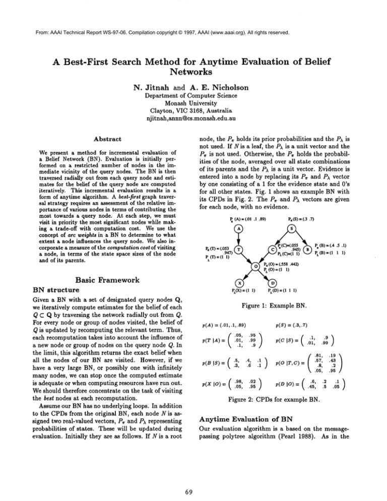
for all other states. Fig. 1 shows an example BNwith
its CPDsin Fig. 2. The P~ and P~ vectors are given
for each node, with no evidence.
Abstract
Wepresent a method for incremental evaluation of
a Belief Network(BN). Evaluation is initially performed on a restricted number of nodes in the immediate vicinity of the query nodes. The BNis then
traversed radially out from each query node and estimates for the belief of the query node are computed
iteratively. This incremental evaluation results in a
form of anytime algorithm. A best-first graph traversal strategy requires an assessmentof the relative importance of various nodes in terms of contributing the
most towards a query node. At each step, we must
visit in priority the mostsignificant nodes while making a trade-off with computation cost. Weuse the
concept of arc weights in a BNto determine to what
extent a node influences the query node. Wealso incorporate a measureof the computationcost of visiting
a node, in terms of the state space sizes of the node
and of its parents.
Basic
p,(s)ffi(.3
P(B) ffi (.4 .5
Px(13)ffi(1 1
Framework
BN structure
Given a BNwith a set of designated query nodes Q,
we iteratively computeestimates for the belief of each
Q c Q by traversing the network radially out from Q.
For every node or group of nodes visited, the belief of
Q is updated by recomputing the relevant term. Thus,
each recomputation takes into account the influence of
a new node or group of nodes on the query node Q. In
the limit, this algorithm returns the exact belief when
all the nodes of our BNare visited. However, if we
have a very large BN, or possibly one with infinitely
many nodes, we can stop once the computed estimate
is adequate or when computing resources have run out.
Weshould therefore concentrate on the task of visiting
the best nodes at each recomputation.
Assumeour BNhas no underlying loops. In addition
to the CPDsfrom the original BN, each node N is assigned two real-valued vectors, P~ and P;~ representing
probabilities of states. These will be updated during
evaluation. Initially they are as follows. If N is a root
69
Figure 1: Example BN.
v(A)= (.01, .t, .S9)
p(T IA)=
v(s) =(.s,.7)
p(C IS) = .01, .99
.01, .99
.9
.I,
.81,
p(B IS)= .3,
.6
( .5,
.4,
p(X
[O)=
.05,
.95
.57,
p(O IT, C)= .S,
.1
.05,
p(D
IO)
= .45,
.5
.19
.43
/
.2
.95
.05
Figure 2: CPDs for example BN.
Anytime Evaluation
of BN
Our evaluation algorithm is a based on the messagepassing polytree algorithm (Pearl 1988). As in the
polytree algorithm, each node N transmits lr and A
messages which are real-valued vectors representing
probabilities of states. Node N sends Ir messages to
its parents and A messages to its children. Consider a
node X which receives 7r messages from parents Z and
A messages from children Y. X updates its P~ and Px
vectors as follows:
(i)
P (X)=
J
P,(X)
-
E CPDx IZ H ~rx(Zi)
i
(2)
An Example
This example shows how the BNof Fig. 1 is evaluated,
with evidence in node X -- 0 and for query node O. We
show the ~r and A messages in Fig. 3 and the anytime
evaluation results in Fig. 4. Wefirst visit the immediate neighbours of O, to get an initial estimate, then
the rest of the BNin depth-first order. In this scenario,
BEL(O)is re-computed after visiting each single node.
The final result for the belief of O is (.733.267), which
is the exact answer. Note that nodes B and D are
pruned because they are independent from the query
node in this situation.
i
Using the messages received, node X computes new
outgoing Ir and/or A messages. See (Pearl 1988) for
more details of the polytree algorithm. Each query
node Q computes its belief by taking the dot product
of P, and P~ vectors and normalising the result as
follows:
r~T(A)
~C(S)
L B(S)
=o(C)
BEL(Q) = a P~(Q) P,,(Q)
~* X (O)
where a is a normalising constant.
For each Q c Q, the first result returned by our
anytime algorithm is an initial estimate of the belief
of Q obtained by collecting messages from its immediate neighbours. Wethen traverse the BNradially out
from Q. Each visted node N will send a message to be
propagated towards Q, which recomputes a more accurate estimate of its ownbeliefs as in Eq. 3. Only the
branches on which visited nodes lie are re-evaluated.
This corresponds to a partial evaluation of Eqs. 2 for
N, with only messages from visited nodes being included.
By visiting a group of nodes, rather than a single
node, at each iteration, we gather more information between successive computations of BEL(Q). The question of howlong to collect information and which nodes
to visit at each stage is the meta-level control problem
of deliberation scheduling, allocating computational resources between two stages (Dean & Wellman 1991,
Ch.8).
The order of traversal
is an important issue.
Breadth-first and depth-first from the query node are
obvious non-heuristic methods. Our best-first strategy
is based on arc weights and also takes into account the
computational cost of visiting a node. Weights of arcs
at a node give an estimate of how much the node can
be affected by each neighbour. Wecan also take into
account the cost, in terms of computation time, of visiting a node. Ideally, we want to make a trade-off by
visiting first the less costly but most influential nodes.
7O
~ D(O)
Figure 3: A and Ir messages in BNwith query O and
evidence X = 0.
Node
T
C
x
A
S
P,,(o)
Px(O) BEL(O)
~o~T)~.OS3.94r~ (.8r81.n2)
1.439.5sl)
~ro(C) (.055.945)
(.n~.s32)
/1111/ (.hr.,,2)
~rp(T
as
above
)
xx(o
.0s)
1.9s.o5)
~.~23.2~)
) (.gs
1.11~.8s2)
~rT(A
.138.864)
(,98.05) (.755.245)
) (.01 .1.89)
~o(T)(.o91.91o)
~rO(G) as above
~rC(S
(.123.37r)
(.ga.0s)
(.r3z.26r)
) (,3,7)
.o(C) (.037.963)
~ro(T)as above
Messagespassed
Figure 4: Anytime evaluation results of BN.
Arc
Weight
and Cost Measures
for
Best-First
Graph Traversal
Arc Weights
The crucial aspect of incremental BNevaluation described above is the order of traversal of the BN. We
want to visit those nodes which have the greatest influence on the query node first. If a node has several
neighbours, we should first consider the one linked by
the strongest connection. The weight of an arc provides an estimate of how much a change in the probability distribution of a node can affect the neighbour
linked by this arc. Given a node Ywith parent Xand a
computing the ~r or A message transmitted. This depends on the size of the CPDof the node. The cost of
collecting a message from node X for its neighbour Y,
which has parents Z, is given by:
set of other parents Z, we calculate the weight w(X, Y)
of the arc X ~ Y as follows:
w(X,Y)-tanh
1
i ~(Z)------
] ~
kea(Z) i,j~a(X)
D(p(Y IX = i, Z = k), p(Y IX = j, Z = k)) (4)
In(r) l (21(x) l
if X sends a A message to Y
DB( P, Q) = -log ~ v/-P~
I fl(Y) [ (2 In(Z)I
if X sends a lr message to Y
In general, for nodes X0 and Xn which are indirectly
connected, we define the path cost C(X0, Xn) of sending a message from X0 to Xn as:
n--1
(5)
c(x, z) = c(x
i
(9)
i=0
Wetake the tanh in Eq. 4 to map the value to the
range (0, 1]. Eq. 4 calculates howmuchthe probabilities of Y will change, as X changes state, averaged over
all state combinations of all other parents. The weight
is computedlocally at each arc because only the values
stored in the CPDfor p(Y IX) are required.
Since messages are also sent from child to parent of
the original BN, a reverse measure of the weight of
an arc is also needed. It is obtained by computing a
CPDfor p(X IY) using Bayes’ Law and repeating the
calculation.
In general, for nodes X0 and Xn which are indirectly
connected, we define the path weight W(Xo, Xn) as:
where Xi+l is the neighbour of X~ on the path to
x..
Best-First
Traversal
Whenusing cost and arc weights to traverse the BN,
each arc is assigned a weight as defined in Eq. 4 and
a cost is assigned to each node as in Eq. 8. To choose
the best node to visit next for query Q, we scan all
unvisited nodes directly connected to visited ones and
select the node N with the largest ratio
W(N, Q)
C(N,Q)
n--1
W(Xo,X.)=
(s)
c(X, Y) =
where fl(N) is the set of states of node N, fl(Z)
is the set of combined states of nodes in Z and D is
a distance between the two probability distributions.
For this purpose, we use the Bhattacharyya (Bhattacharyya 1943) distance between two distributions
and Q. It is given by
(10)
In this way, we bias the search towards the node
which most largely influences our query node, while
making a trade-off with computational cost. Fig. 5
shows the cost and arc weights of our example BN,
with query node O.
(6)
i----0
where Xi+t is the neighbour of X/on the path to Xn.
Taking the product over all arc weights on the path
between X and Xn gives a measure of the combined
effect of the intervening nodes and takes into account
the distance between X and Xn, thus incorporating
the impact of topological proximity and relevance described in (Poh & Horvitz 1996).
Note that our weight measure is suitable for multistate nodes. In the case of binary nodes, it is simpler
to use the connection strength measure introduced in
(Boerlage 1995), from which ours was inspired:
w = 201
c=24
w = .006
c=20
w= 7e-5
~30
w= .10~
c=
w = .779
c=6
w= .239
14
w -- .022
c=10
CS(A, B) = log p(b la) log p(b I’~a)
p(’~b I-~a) (7)
p(’~b la)
Cost of Visiting
a Node
Figure 5: BNshowing path weight and path cost for
query O.
Wecalculate the cost of visiting a node in terms of
the number of additions and multiplications done when
71
Experimental
Results
curve for arc weights curve.
The experimental results given in this section involve
a polytree network of 22 nodes, shown in Fig. 6. It
is adapted from the example in (Boerlage 1995).
evaluate the BNusing breadth-first,
depth-first and
best-first strategies. Wecalculate an initial estimate
of the posterior of our query node by visiting its direct
neighbours. At each subsequent single node visit, we
update the posterior of the query node and calculate
the error in the result in terms of the Kullback-Leibler
(KL) distance (Pearl 1988) between the current estimate and the exact value. Note that we initially evaluated the network using a join-tree algorithm (Lauritzen
& Spiegelhalter 1988) to obtain the exact answer. For
illustration purposes, we recomputed the posterior of
the query node after every single node visit. Normally,
it is preferable to visit a group of nodes at each iteration to minimise overheads and increase the rate of
improvement in result accuracy.
’ Depth~nt
Breadth
F~rst
AmWelgMs
-s--.
0.00025
|
0.0C02
~ 0.00015
|
0.0001
0
0
2
&’""
’
""
"~-’~
.........
4
6
8
10
12
14
16
STEPS
IN EVALUATION
OFBNgrs4~h
{Number
of NOdes
Ir~luded)
t
18
Figure 7: Comparison of graph traversal strategies:
Breadth-First, Depth-First and Best-First (using Arc
Weights).
Discussion
Belief networks have been used in applications that require real-time monitoring of complex domains, where
the cost of computingan exact solution is prohibitive.
Anytime algorithms have been developed for such
problems. The approach described here regards BN
evaluation as a search problem under limited resources.
Evaluation is initially performed on a restricted number of nodes in the immediate vicinity of the query
nodes. The BNis then traversed radially out from the
query node and estimates for the belief of the query
node are computediteratively, i.e. after visiting a new
node or group of nodes.
At each search step search, there is a result accuracy vs computation cost trade-off. The cost C(N, Q)
of visiting a node N and correspondingly updating
the query node Q represents computational complexity. Our measure of path weights gives the strength
of the connection W(N,Q) between N and Q; this
correponds to the improvement in the accuracy of our
result. Our best-first strategy chooses to visit in priority node with the largest
ratio ~. Hence the
search is biased in favour of more significant but less
costly nodes.
We cannot obtain an exact run-time assessment of
the solution quality at each step. But we have an estimate of any node’s influence on the query node, in
terms of the path weight. In general, visiting nodes
on heavier paths gives rise to faster improvement in
the result. Our cost measure can be used for run-time
allocation of computational resources. With limited
Figure 6:22 node polytree, adapted from the example
in [3], used to obtain experimental results. Query node
is shaded and evidence node shown in bold.
Fig. 7 shows the performances of breadth-first,
depth-first and best-first /w(g,q)~ strategies. HH
C(N,Q)
thequerynodeand theevidence
nodeis FW. Themajordip in the curves occurs when node PAis visited.
This large fall in the error shows that PAhas a great
influence on our query node. Because arc PA ---* PC
has a large weight, our best-first strategy chooses to
visit PAfirst. This is indicated by the early drop in the
72
time and memoryat each step, we look at the cost
of visiting some nodes to decide if the computation is
feasible. Then, we want to select the most profitable
group of nodes to include in our computation, given the
amount of resources available. This is the meta-level
control problem of deliberation scheduling.
Our current algorithm is a greedy search because it
only chooses the next best option at each step. An
issue to consider is howto perform a search with lookahead, i.e. not just choosing the current best node,
but the one leading to the most significant region of
the BN, in terms of influence on the query node. For
this purpose, we would need to develop a measure of
the total weight of a section of the BNconsisting of
multiple branches diverging from a given node.
The procedure presented here does not strictly satisfy all the ideal requirements of anytime algorithms
stated in (Zilberstein 1995). Wecan obtain a measurable quality of result only by comparing the output to
the exact result which will not be available at run-time.
While we can show empirically that in most cases, on
average, the algorithm produces more accurate results
over time, we cannot guarantee monotonicity. Our algorithm is fully interruptible. In this paper, we have
shown how to apply our algorithm to BNs which are
polytree structures. Since most BNswith underlying
loops can be converted to clique-trees our formulation
can be adapted to suit a larger category of structures.
References
Bhattacharyya, A. 1943. On a measure of divergence
betweentwo statistical populations defined by their probability distributions. Bulletin of the Calcutta Mathematics
Society 35:99-110.
Boerlage, B. 1995. Link strengths in bayesian networks.
Master’s thesis, Dept. of ComputerScience, U. of British
Columbia.
Dean, T., and Wellman,M. P. 1991. Planning and control.
San Mateo, Ca.: MorganKaufmanPublishers.
Lauritzen, S., and Spiegelhalter, D. 1988. Local computations with probabilities on graphical structures and
their applications to expert systems. Journal of the Royal
Statistical Society 50(2):157-224.
Pearl, J. 1988. Probabilistic ReasoningIn Intelligent Systems: Networks of Plausible Inference. Morgan Kaufmann.
Poh, K. L., and Horvitz, E. 1996. Topological proximity
and relevance in graphical decision models. In Proc. of
l~th Conf. on UAI, 427-435.
Zilberstein, S. 1995. Compositionand monitoring of anytime alforithms. In IJCAI 95: Anytime Algorithms and
Deliberation Scheduling Workshop,14-21.
73