From: KDD-95 Proceedings. Copyright © 1995, AAAI (www.aaai.org). All rights reserved.
Decision
Tree Induction:
Sreerama
How Effective
Murthy
and
Steven
is the Greedy Heuristic?
Salzberg
Department of Computer Science
Johns Hopkins University
Baltimore, Maryland 21218
lastname@cs.jhu.edu
Abstract
Mostexisting decision tree systems use a greedy approachto inducetrees -- locally optimalsplits are inducedat every node of the tree. Althoughthe greedy
approachis suboptimal,it is believed to producereasonablygoodtrees. In the current work, weattempt to
verify this belief. Wequantify the goodnessof greedy
tree induction empirically, using the popular decision
tree algorithms, C4.5 and CART.Weinduce decision
trees on thousands of synthetic data sets and compare them to the corresponding optimal trees, which
in turn are found using a novel mapcoloring idea. We
measurethe effect on greedy induction of variables
such as the underlying concept complexity, training
set size, noise and dimensionality. Our experiments
show, amongother things, that the expected classification cost of a greedily induced tree is consistently
very close to that of the optimal tree.
Introduction
Decision trees are knownto be effective classifiers in
a variety of domains. Most of the methods developed
have used a standard top-down, greeay approach to
building trees, which can be summarized as follows.
Recursively do the following until no more nodes can
be split: choose the best possible test at the current
node according to some goodness measure and split the
current node using that test; after a complete tree is
grown, prune it back to avoid overfitting the training
data (Breiman et al. 1984; Quinlan 1993). The choice
of a "best" test is what makes this algorithm greedy.
The best test at a given internal node of the tree is
only a locally optimal choice; and a strategy choosing
locally optimal splits necessarily produces suboptimal
trees (Goodman & Smyth 1988).
Optimality of a decision tree may be measured in
terms of prediction accuracy, size or depth. It should
be clear that it is desirable to build optimal trees in
terms of one or more of these criteria.
Maximizing
classification accuracy on unseen data (within the constraints imposedby the training data) is obviously desirable. Smaller, shallower decision trees imply better
comprehensibility and computational efficiency. Shallow trees are also more cost-effective, as the depth of
222
KDD-95
a tree is a measure of its classification
cost. However, because the problem of building optimal trees
is known to be intractable (Hyafil & Rivest 1976;
Murphy & McCraw1991), a greedy heuristic
might
be wise given realistic computational constraints.
The goal of this paper is to examineclosely the consequences of adopting a greedy strategy. Weask the
question, if we had unlimited resources and could compute the optimal tree, how much better should we expect to perform? An alternative
way of asking the
same question is, what is the penalty that decision tree
algorithms pay in return for the speed gained by the
greedy heuristic?
Setting
up the Experiments
Our experimental framework is quite simple -- we use
C4.5 (Quinlan 1993) and CART(Breiman et al. 1984)
to induce decision trees on a large number of random
data sets, and in each case we compare the greedily
induced tree to the optimal tree. The implementation
of this frameworkraises someinteresting issues.
Optimal Decision Tree for a Training Set. The
problem of computing the shallowest or smallest decision tree for a given data set is NP-complete(Hyafil
Rivest 1976; Murphy & McCraw1991), meaning that
it is highly unlikely that a polynomial solution will be
found. Previous studies that attempted comparisons
to optimal trees (e.g., (Cox, Qiu, & Kuehner 1989))
used approaches like dynamic programming to generate the optimal trees. Becauseit is slow, this option is
impractical for our study, in which we use hundreds of
thousandsof artificial data sets. Oursolution is to first
generate a random decision tree D, and then generate
data sets for which D is guaranteed to be the optimal
tree. The main idea behind ensuring the optimality of
a randomdecision tree is coloring its leaf nodes with
appropriate class labels.
An instance
is a real valued vector Xi =
(x~l,zi2,...,xia)
plus a class label c~. xis are the attributes of Xi, and d is its dimensionality. Consider a
binary decision tree D in two attributes. (The ensuing
argument applies to arbitrary dimensions.) D induces
a hierarchical partitioning of the attribute space, which
can be drawn as a map M. The boundaries of M are
the splits (test nodes) in D, and the regions of Mare
the leaf nodes in D. Assumingthat each leaf node of
D contains instances of only one class, we can color M
by assigning a distinct color to each class in D. Now
consider a data set S consistent with D, which has
the additional property that S requires every leaf node
of D, i.e., every leaf node of D contains at least one
instance of S.
It should be clear that D is the smallest binary decision tree consistent with S, provided no two neighboring regions of Mhave the same color. Informally,
any decision tree that has fewer leaves than D needs
to either ignore some decision regions of D, or merge
(parts of) two or more regions into one. The former
possibility is ruled out because S requires all decision
regions in D. The latter is impossible because no decision regions of the same color are adjacent, so no two
regions can be merged. Hence, any decision tree consistent with S has to have at least as manyleaf nodes
as D. Moreover, if D was a perfectly balanced tree to
start with, then any decision tree consistent with S has
to be at least as deep as D.
In our experiments, we start with perfectly balanced,
empty trees. We then generate random tests at the
decision nodes, ensuring that no leaf region is empty.
Finally we color the leaves to ensure optimality with
respect to size, using the following procedure. Wefirst
compute the adjacency information of the leaf nodes.
After initializing the class labels at all leaf nodes to k
(> number of leaves), we go back and change the label
of each leaf to be the smallest numberin [1, k] that is
not yet assigned to any neighbor. This heuristic procedure worked quite well in all our experiments. (For
instance, decision trees of 64 leaf nodes in the plane
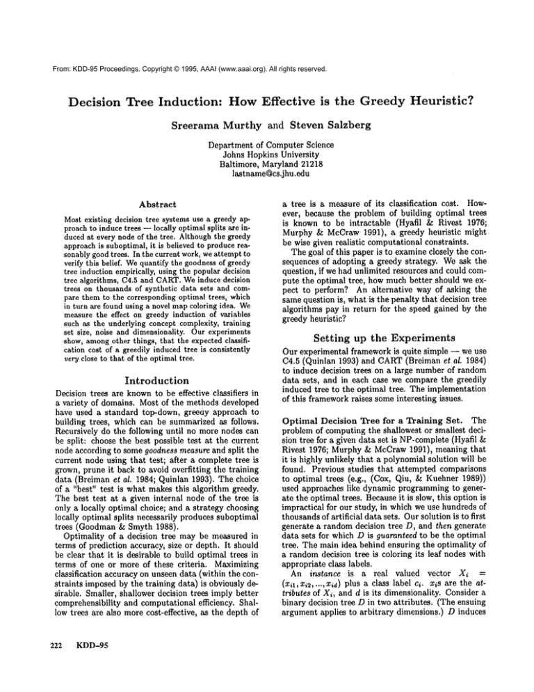
were colored with 5 classes on average.) A sample randomdecision tree in 2-D, along with the class labels
assigned by the above coloring procedure, is shown in
Fig. 1.
Tree Quality Measures. In all our experiments,
report tree quality using six measures:
we
¯ Classification accuracy: accuracy on the training
data;
¯ Prediction accuracy: accuracy on an independent,
noise-free testing set;
¯ Tree size: numberof leaf nodes;
¯ Maximumdepth: distance from the root to the farthest leaf node; (distance from A to B is the number
of nodes between, and including, A and B)
¯ Average depth: mean distance from the root to a
leaf node in the tree;
¯ Expected depth: number of tests needed to classify
an unseen example. Wecompute expected depth by
averaging, over all the examples in the testing set,
2
2
1
1
2
Figure 1: The partitioning induced by a random decision tree of 32 leaf nodes. Class labels assigned by our
coloring procedure are shown (for most nodes).
the length of the path that the example followed in
the tree.
Control Variables. The effectiveness of greedy induction can not be measured independently of training
data characteristics. For instance, if the training data
is very noisy, it is likely that no induction methodwill
be able to generate accurate trees. In this paper, we
study the effectiveness of greedy induction in controlled
settings with respect to the following parameters:
¯ concept complexity (measured as the size of the optimal decision tree),
¯ size of the training set,
¯ amount and nature of noise in the training data
(noise in class labels versus noise in attributes), and
¯ dimensionality (number of attributes).
Tree Induction Methods Used. The tree induction
methods we use are C4.5 (Quinlan 1993) and CART
(Breiman et al. 1984). One main difference between
C4.5 and CARTis the goodness criterion, the criterion
used to choose the best split at each node. C4.5 uses
the information gain 1 criterion, whereas CARTuses
either the Gini index of diversity or the twoing rule. All
the experiments in this paper were repeated using information gain, Gini index and twoing rule. In no case
did the results showstatistically significant differences
between goodness measures--the differences in accuracies, sizes and measurements of depth were always
much less than one standard deviation. For brevity,
we report only the results with information gain (i.e.,
C4.5) in the rest of this paper. Weimplemented all
the goodness measures using the OC1system (Murthy,
1Quinlan suggested gain ratio as an improvementover
information gain. Howeverthe two measuresare equivalent
in our experimentsas all our decision trees are binary.
Murthy
223
Optimal
Size
8
16
32
64
Training
Set
1000
1000
1000
1000
Classification
Accuracy
100.0
100.0
100.0
100.0
Prediction
Accuracy
99.54-0.1
98.74-0.3
97.24-0.6
94.34-0.9
Tree Size
9.84-1.7
20.74-3.3
40.4-t-6.8
71.74-10.3
Maximum
4.84-0.7 (3)
7.24-1.0 (4)
9.3=t=1.0(5)
11.54-1.2 (6)
Depth
Average
3.6=1=0.3(3)
5.0=t=0.4(4)
6.34-0.5 (5)
7.4-t-0.5 (6)
Expected
2.94-0.3 (3)
3.94-0.4 (4)
5.0+0.5(5)
5.84-0.5
(6)
Table 1: Effects of concept complexity. No noise in data. Numbersin parentheses are for the optimal trees.
Kasif, & Salzberg 1994). Although C4.5 and CART
differ in respects other than the goodness measures, we
have not implementedthese differences. In the experiments in which the training data is noise-free, no pruning was used with either method. In the experiments
using noisy training sets, we augment both methods
with cost complexity pruning (Breiman et al. 1984),
reserving 10%of the training data for pruning.
Experiments
This section describes five experiments, each of which
is intended to measure the effectiveness of greedy induction as a function of one or more control variables
described earlier. The procedure is more or less the
same for all experiments.
For each setting of the control variables:
generate 100 random trees with no class labels;
for each tree Dom generated in the above step:
color Dopt with class labels;
generate a large, noise-free testing set
for which Dom is optimal;
generate 50 training sets using Dopt;
for each training set T:
greedily induce a tree D on T;
record D and Dopt;
report the mean and std. dev. of the quality
measures for the 5000 trees.
The instances in the training and testing sets are
always generated uniformly randomly, and are labeled
using the optimal decision tree. The size of the testing
set is linearly dependent on the complexity of the optimal tree and the dimensionality of the data, whereas
the size of the training set is a control variable. More
precisely, [T[ = C * (D - 1) * 500, where [T[ is the size
of the testing set, C is the size of the optimal tree and
D is the numberof attributes. For instance, for a size
16 concept in 4 dimensions, we use a testing set of size
16 ¯ (4 - 1) * 500 = 24,000. Weensure that no subtree of the optimal decision tree is consistent with the
testing set.
In all the tables in this paper, each entry comprises
of the average value of a tree quality measureover 5000
trees and the standard deviation (one a). Numbers
parentheses correspond to the optimal trees. The a’s
are omitted when they are zero. Optimal values are
omitted when their values are obvious. The optimal
trees always give 100%prediction accuracy in our ex-
224
KDD-95
periments, because the testing set has no noise. In
addition, they give 100%classification accuracy when
the training data is noise-free.
Experiment 1: The purpose of this experiment is
to evaluate the effectiveness of greedy induction as a
function of the size of the optimal tree. All training
sets comprise of 1000 random 2-D instances. There is
no noise in the training data. Table 1 summarizesthe
results.
Observations: The prediction accuracy of greedily
induced trees decreases as the size of the optimal tree
for the data increases. This can be either be due to
the inadequacy of greedy search or due to inadequate
training data. (The training set size remained at 1000
though the concept complexity increased from 8 to 64.)
In Experiment 2, we increase the size of the training
set in proportion with the size of the optimal tree, in
order to better isolate the effects due to greedy search.
The difference between the sizes of greedily induced
and optimal trees increases with the size of the optimal
tree in Table 1. However, it can be seen on closer
observation that the variances, not just the differences
in size, are increasing. Greedily induced tree sizes are
just more than one a away from the optimal in 3 out of
4 rows, and less than one std. dev. away for concepts
of size 64.
The maximumdepth measurements in Table 1 show
that greedily induced trees can have decision paths
which are about twice as long as those in the optimal
trees, even for moderately complex concepts. However,
the average depth measurements show that the decision paths in greedily induced trees only have about
one test more than those in the optimal trees. In terms
of the third depth measurement, the expected depth,
greedily induced trees are almost identical to the optimal ones, for all the concept sizes considered in this
experiment. This is a very desirable, although somewhat counterintuitive, trend which is seen consistently
throughout our experiments. (Note that no pruning
was used in this experiment.)
Experiment 2: The purpose of this experiment is to
isolate the effects of concept complexity, from those
of the training set size. The size of the training sets
now grows linearly with the concept complexity--25
training points on average are used per each leaf of the
optimal tree. There is no noise. Table 2 summarizes
Optimal
Size
8
16
32
64
Training
Set
200
4OO
800
1600
Classification
Accuracy
100.0
100.0
100.0
100.0
Prediction
Accuracy
97.5+0.7
97.1±0.7
96.64-0.7
96.4±0.6
Tree Size
8.5±1.5
17.5±3.3
38.04-7.1
76.3±12.3
Maximum
4.4=1=0.6(3)
6.6±0.9 (4)
9.1±1.0 (5)
11.6=t=1.2(6)
Depth
Average
3.4+0.3 (3)
4.7±0.5 (4)
6.2±0.5 (5)
7.5±0.6 (6)
Expected
2.84-0.3 (3)
3.8±0.5 (4)
4.S±0.5 (5)
5.8±0.6 (6)
Table 2: Effects of concept complexity and training set size. No noise. Numbersin parentheses are for the optimal
trees.
Class
Noise
Classification
Accuracy
o%
loo.o (loo.o)
5% 92.1±1.3 (95.1±0.01)
lO% 87.7±1.3 (90.5-4-0.02)
15%
20%
25%
83.5+1.3 (86.1±0.05)
79.7±1.4 (81.9±0.05)
76.14-1.4 (77.8+0.03)
Prediction
Accuracy
93.9±1.4
89.5±2.4
88.2-1-2.6
86.6±2.9
84.9±3.1
83.14-3.4
Tree Size
31.14-6.2
21.9±5.1
22.24-5.1
22.4±5.4
22.7±5.2
23.34-5.7
Maximum
8.2±0.9
7.0±0.8
7.0±0.8
7.0+0.8
7.1±0.8
7.14-0.8
Depth
Average I Expected
5.6±0.4I 4.8±0.5
4.9±0.5
4.4±0.4
4.9+0.4
4.4±0.4
4.9-t-0.5
4.4±0.4
4.9±0.5
4.4±0.4
4.8±0.5
4.4±0.4
Table 3: Effects of noise in class labels. Numbersin parentheses are for the optimal trees. Optimal trees are of size
32.
the results.
Observations: It is interesting to note that the prediction accuracy does not drop as muchwith increase
in optimal tree size here as it does in Experiment 1.
In fact, when the optimal trees grew 8 times as large
(from 8 to 64), the accuracy went down by just more
than one standard deviation. In addition, none of the
differences in tree size between greedily induced and
optimal trees in Table 2 are more than one a. This
is surprising, considering no pruning was used in this
experiment. In terms of the three depth measures, the
observations made in Experiment 1 hold here also.
Comparingthe entries of Tables 1 and 2, line by line,
one can see the effect of the training set size on prediction accuracy. Whenthe training set size increases,
the prediction accuracy increases and its variance goes
down. In other words, the more (noise-free) training
data there is, the more accurately and reliably greedy
induction can learn the underlying concept.
Experiment 3: This experiment is intended to evaluate the effectiveness of greedy induction in the presence
of noise in class labels. The training sets are all in 2-D,
and consist of 100 instances per class, uniformly randomlydistributed in each class, k%noise is added into
each training set by incrementing by 1 the class labels
of a random k% of the training points. All concepts
are of size 32, so all optimal tree depth values are equal
to 5.0. Pruning was used when noise level is greater
than 0%. Table 3 summarizes the results.
Observations: As is expected, the classification and
prediction accuracies decrease when the amount of
noise is increased. The tree size and and depth measurements vary significantly whenthe first 5%of noise
is introduced (obviously because pruning is started),
and remain steady thereafter.
One needs to be careful in analyzing the results of
experiments 3 and 4, in order to separate out the effects of noise and the effect of the greedy search. What
we want to investigate is whether the greedy heuristic
becomesless and less effective as the noise levels increase, or if it is robust. For instance, the fact that
the classification accuracy decreases linearly with increase in noise in Table 3 is perhaps not as significant
as the fact that the prediction accuracy decreases more
slowly than classification accuracy. This is because the
former is an obvious effect of noise whereas the later
indicates that greedy induction might be compensating
for the noise.
Several patterns in Table 3 argue in favor of the effectiveness of pruning, which has come to be an essential
part of greedy tree induction. Classification accuracies
of the greedy trees are close to, and less than, those
of the optimal trees for all the noise levels, so overfitting is not a problem. Prediction accuracies of greedily
induced trees with pruning are better than their classification accuracies, again indicating that there is no
strong overfitting. Tree size and depth measurements
remained virtually unchanged in the presence of increasing noise, certifying to the robustness of pruning.
Experiment 4: This experiment is similar to the
previous one, in that we measure the effectiveness of
greedy induction as a function of noise in the training
data. However,this time we consider noise in attribute
values. The training sets again comprise 100 2-D instances per class, uniformly randomly distributed in
each class, k%noise is introduced into each training
Murthy 225
Attribute
Noise
0%
5%
10%
15%
20%
25%
Classification
Accuracy
Prediction
Accuracy
93.94-1.4
lOO.O
(loo.o)
90.04-2.3
95.24-1.3 (08.04-0.4)
88.74-2.6
93.5+1.4 (96.04-0.7)
92.14-1.6 (94.14-1.0)
87.44-2.8
90.7+1.8 (92.25=1.3)
86.24-3.1
89.45=2.0
(9o.6+1.~) 85.04-3.4
Table 4: Effects of noise in attribute
size 32.
#Dim.
2
4
8
12
Classification
Accuracy
I00.0
I00.0
100.0
100.0
Tree Size
Depth
Maximum [ Average Expected
31.14-6.2
8.24-0.9
5.64-0.4
4.84-0.5
22.24-5.3
7.04-0.8
4.94-0.5
4.44-0.4
22.65=5.5
7.0±0.8
4.94-0.5
4.44-0.4
23.35=5.6 7.05=0.8 5.05=0.5 4.45=0.4
23.74-5.6
4.94-0.5
4.45=0.4
7.04-0.8
4.35=0.4
23.75=5.5
7.05=0.8
4.94-0.5
values. Numbersin parentheses are for optimal trees. Optimal trees are of
Prediction Tree Size
Depth
Accuracy
MaximumI Average [ Expected.
7.24-1.0
5.0+0.4
3.94-0.4
98.75=0.320.75=3.3
98.34-0.7
23.95=6.0 6.65=0.9
5.04-0.5
4.05=0.4
98.05=0.8 24.54-6.5
6.34-0.9
4.94-0.5
4.15=0.2
97.94-0.9
25.45=6.8 6.34-0.9
4.94-0.5
4.15=0.2
I
Table 5: Effects of dimensionality. Training set size=1000. No noise. Optimal trees are of size 16.
set by choosing a random k% of the instances, and by
adding an e E [-0.1,0.1] to each attribute. All the
concepts are of size 32, so all the optimal depth measurements are equal to 5.0. Cost complexity pruning
was used in cases where the noise level was greater than
0%. The results are summarized in Table 4.
Observations: There results with attribute noise (Table 4) and noise in class labels (Table 3) are very similar, except for the classification accuracies. The values
for prediction accuracy, tree size and depth measurements in the presence of k%noise are almost the same
whether the noise is in attribute values or class labels.
The classification and prediction accuracies decrease
with increasing noise. The tree size and depth measurements decrease when the first 5%of the noise is
introduced (due to pruning) and remain steady thereafter.
However, introducing k% attribute
noise is not
equivalent to introducing k% class noise. Changing
the attributes of an instance by a small amountaffects
the classification of only those instances lying near the
borders of decision regions, whereas changing the class
labels affects the classification of all the instances involved. This can be seen from the classification accuracies of the optimal trees in Tables 3 and 4. The
classification accuracy of the greedy trees is quite close
to, and less than that of the optimal trees in both
tables. All the prediction accuracy values in Table 4,
unlike those in Table 3, are less than the corresponding
classification accuracies.
Experiment 5: Our final experiment attempts to
quantify the effect of dimensionality on the greedy
heuristic. All the training sets consist of 1090 uniformly randomly generated instances, wish no noise,
226
KDD-95
as in Experiment 1. No pruning was used. All concepts are of size 16, so the optimal tree depths are 4.0.
Table 5 summarizes the results.
Observations: The changes in all tree quality measures are quite small when dimensionality is increased
from 2 to 12. This result is surprising because, intuitively, higher dimensional concepts should be much
more difficult to learn than lower dimensional ones,
when the amount of available training data does not
change. Our experiments indicate that the effects due
to dimensionality do not seem to be as pronounced
as the effects due to concept complexity (Table 1)
noise. The quantity that does increase with increasing
dimensionality is the variance. Both prediction accuracy and tree size fluctuate significantly morein higher
dimensions than in the plane. This result suggests that
methods that help decrease variance, such as combining the classifications of multiple decision trees (see
(Murthy 1995) for a survey), may be useful in higher
dimensions.
Discussion and Conclusions
In this paper, we presented five experiments for evaluating the effectiveness of the greedy heuristic for decision tree induction. In each experiment, we generated
thousands of random training sets, and compared the
decision trees induced by C4.5 and CARTto the corresponding optimal trees. The optimal trees were found
using a novel graph coloring idea.
Wesummarize the main observations from our experiments below. Where relevant, we briefly mention
related workin the literature.
¯ The expected depth of greedily induced decision trees
was consistently very close to the optimal. Garey
¯
¯
¯
¯
¯
and Graham (1974) showed that a recursive greedy
splitting algorithm using information gain (not using
pruning) can be made to perform arbitrarily
worse
than the optimal in terms of expected tree depth.
Goodmanand Smyth (1988) argued, by establishing the equivalence of decision tree induction and a
form of Shannon-Fanoprefix coding, that the average depth of trees induced by greedy one-paas (i.e.,
no pruning) algorithms is nearly optimal.
Cost complexity pruning (Breiman et 02. 1984) dealt
effectively with both attribute and class noise. However, the accuracies on the training set were overly
optimistic in the presence of attribute noise.
Greedily induced trees became less accurate as the
concepts becameharder, i.e., as the optimal tree size
increased. However,increasing the training data size
linearly with concept complexity helped keep the accuracy stable.
Greedily induced trees were not much larger than
the optimal, even for complex concepts. However,
the variance in tree size was more for higher dimension02 and more complex concepts. Dietterieh and
Kong(1995) empirically argued that even in terms
of prediction accuracy, variance is the main cause for
the failure of decision trees in somedomains.
For a f~ed training set size, increasing the dimension02ity did not affect greedy induction as much as
increasing concept complexity or noise did. Several
authors (e.g., (Fukanaga & Hayes 1989)) have
gued that for a finite sized data with no a priori
probabilistie information, the ratio of training sample size to the dimensionality must be aa large aa
possible. Our results are consistent with these studies. However, with a reasonably large training set
(1000 instances), the drop in tree quality was quite
small in our experiments, even for a 6-fold (2 to 12)
inereaae in dimensionality.
The goodness measures of CART and C4.5 were
identical in terms of the quality of trees they generatetL It has been observed earlier (e.g.,(Breiman
et 02. 1984; Mingers 1989)) that the differences between these goodness criteria are not pronounced.
Our observation that these measures consistently
produced identical trees, in terms of six tree quality measures, in a large scale experiment (involving
more than 130,000 s~rnthetic data sets) strengthens
the existing results. --
improve upon the simple greedy algorithm for decision
tree induction.
References
Breiman, L.; Friedman, J.; Olshen, R.; and Stone, C.
1984. Classification and Regression Trees. Wadsworth
International Group.
Cox, L. A.; Qiu, Y.; and Kuehner, W. 1989. Heuristic
leaat-cost computationof discrete classification functions with uncertain argument values. Annals of Operations Research 21(1):1-30.
Dietterieh, T. G., and Kong, E. B. 1995. Machine
learning bias, statistical bias and statistical variance
of decision tree algorithms. In Machine Learning:
Proceedings of the Twelfth International Conference.
Tahoe City, CA: Morgan Kanfmann Publishers Inc.,
San Mateo, CA. to appear.
Fukanaga, K., and Hayes, tLA. 1989. Effect of sample
size in elaasifier design. IEEE Transactions on Pattern Analysis and MachineIntelligence 11:873-885.
Garey, M. R., and Graham, R. L. 1974. Performance
bounds on the splitting algorithm for binary testing.
Acta Informatica 3(Fase. 4):347-355.
Goodman, R. M., and Smyth, P. J. 1988. Decision tree design from a communication theory standpoint. IEEE Transactions on Information Theory
34(5):979-994.
Hyafil, L., and Rivest, 1~ L. 1976. Constructing optimal binary decision trees is NP-complete. Information Processing Letters 5(1):15--17.
Mingers, J. 1989. An empirical comparison of selection measures for decision tree induction. Machine
Learning 3:319-342.
Murphy, O. J., and McCraw, R. L. 1991. Designing
storage efficient decision trees. IEEETransactions on
Computers 40(3):315-319.
Murthy, S. K.; Kasif, S.; and Salzberg, S. 1994. A
system for induction of oblique decision trees. Journal
of Artificial Intelligence Research2:1-33.
Murthy, S.K.
1995. Data exploration
using decision trees: A survey. In preparation.
http://www.es.jhu.edu/grad/murthy.
Quinlan, J. R. 1993. C4.5: Programs for Machine
Learning. San Mateo, CA: Morgan Kaufmann Publishers.
Manyresearchers have studied ways to improve upon
greedy induction, by using techniques such aa limited
lookahead search and more elaborate classifier representations (e.g., decision graphs instead of trees). (See
(Murthy 1995) for a survey.) The results in the current paper throw light on whyit might be difficult to
2The fact that we only used binary splits in reabvalued
domains may be one reason why information gain, Gini
index and twoing rule behavedsimilarly.
Murthy
227