From: KDD-95 Proceedings. Copyright © 1995, AAAI (www.aaai.org). All rights reserved.
‘?J/,‘:
,, /”
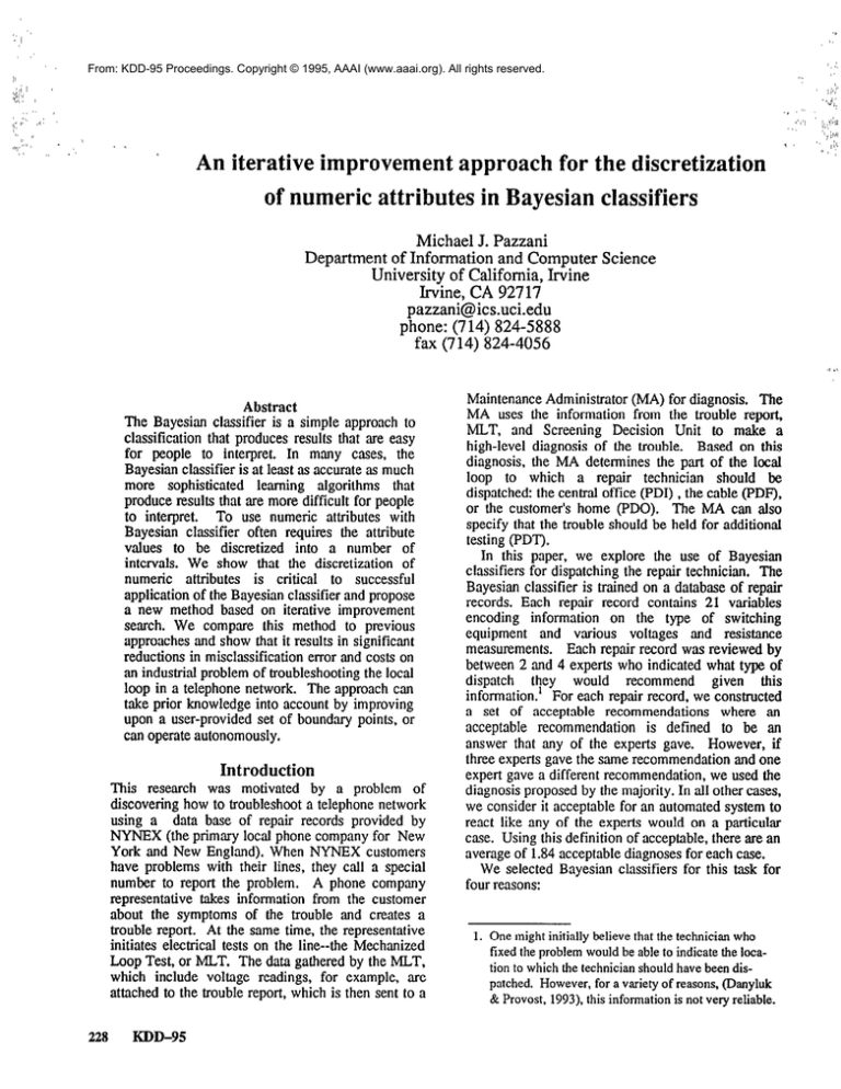
8’/‘/
I,,
0
An iterative improvement approach for the discretization
of numeric attributes in Bayesian classifiers
M ichael J. Pazzani
Department of Information and Computer Science
University of California, Irvine
Irvine, CA 92717
pazzani@ics.uci.edu
phone: (714) 824-5888
fax (714) 824-4056
Abstract
The Bayesian classifier is a simple approach to
classification that produces results that are easy
for people to interpret. In many cases, the
Bayesian classifier is at least as accurateas much
more sophisticated learning algorithms that
produce results that are more difficult for people
to interpret. To use numeric attributes with
Bayesian classifier often requires the attribute
values to be discretized into a number of
intervals. W e show that the discretization of
numeric attributes is critical to successful
application of the Bayesianclassifier and propose
a new method based on iterative improvement
search. W e compare this method to previous
approachesand show that it results in significant
reductions in m isclassification error and costs on
an industrial problem of troubleshootingthe local
loop in a telephonenetwork. The approachcan
take prior knowledge into account by improving
upon a user-providedset of boundary points, or
can operateautonomously.
Introduction
This research was motivated by a problem of
discovering how to troubleshoota telephonenetwork
using a data base of repair records provided by
NYNEX (the primary local phone company for New
York and New England). W h e n NYNEX customers
have problems with their lines, they tail a special
number to report the problem. A phone company
representativetakes information from the customer
about the symptoms of the trouble and creates a
trouble report. At the same time, the representative
initiates electrical tests on the line--the Mechanized
Loop Test, or Iv&T. The data gatheredby the MLT,
which include voltage readings, for example, are
attachedto the trouble report, which is then sent to a
228
KDD-95
M a intenanceAdministrator (MA) for diagnosis. The
MA uses the information from the trouble report,
MLT, and Screening Decision Unit to make a
high-level diagnosis of the trouble. Based on this
diagnosis, the MA determines the part of the local
loop to which a repair technician should be
dispatched:the central office (PDI) , the cable (PDF),
or the customer’sh o m e (PDO). The MA can also
specify that the trouble should be held for additional
testing (PDT).
In this paper, we explore the use of Bayesian
classifiers for dispatching the repair technician. The
Bayesian classifier is trained on a databaseof repair
records. Each repair record contains 21 variables
encoding information on the type of switching
equipment and various voltages and resistance
measurements. Each repair record was reviewed by
between 2 and 4 experts who indicated what type of
dispatch they would recommend given this
information.’ For each repair record, we constructed
a set of acceptable recommendations where an
acceptable recommendation is defined to be an
answer that any of the experts gave. However, if
three experts gave the samerecommendationand one
expert gave a different recommendation,we used the
diagnosisproposedby the m a jority. In all other cases,
we consider it acceptablefor an automatedsystem to
react like any of the experts would on a particular
case. Using this definition of acceptable,there are an
averageof 1.84 acceptablediagnosesfor each case.
W e selected Bayesian classifiers for this task for
four reasons:
1. One might initially believe that the technician who
fixed the problem would be able to indicate the location to which the technician should have been dispatched. However, for a variety of reasons, (Danyluk
& Provost, 1993), this information is not very reliable.
;,,rh
‘/
‘&;!11/
” ,i;
”
1. It has been found that they can be at least as
accurate as more “sophisticated” learning
methods (e.g., Kononenko, 1990).
2. Bayesian classifiers produce an estimate of the
probability that an example belongs to each
class. This probability estimate may be used to
determine the most likely class of a training
example, or the class that will have the least
expected cost of misclassification errors. While
other learners (e.g., decision trees, Quinlan,
1986) may be extended to produce probability
estimates, in practice, these estimates do not vary
continuously and do not provide fine-grained
information to perform well at determining the
least expected cost of misclassification errors
(e.g., Pazzani, Merz, Murphy, Ali, Hume,
and Brunk, 1994).
3. The Bayesian classifier reveals information that
some experts find more useful than other models
such as decision trees (Kononenko, 1991). The
results of the Bayesian classifier are conditional
probabilities that may be viewed as simple, one
attribute rules.
4. It is possible to take advantage of expert
a---...l-1-_- ALKuowieoge on
me criiicai vaiues of continuous
variables, and revise this information, as we shall
describe.
However, on some problems, the simple Bayesinn
classifier is much less accurate than other learners. In
Pazzani (1995), we addressed one possible problem
with Bayesian classifiers in that they assume attribute
values are independent within each class. However,
the methods used to detect and correct for violations
of this assumption did not have an effect on the
accuracy or misclassification cost of the Bayesinn
classifier on the telephone troubleshooting database.
In this paper, we address another problem with using
Bayesian classifiers on practical problems: the
treatment of numeric data. We also address issues
that occur when learning from data in which there is
disagreement among experts and exploiting
information from experts on how numeric data may
be discretized.
Background
The Bayesian classifier (Duda Jc Hart, 1973) is a
probabilistic method for classification. It can be used
to determine the probability that an example j
belongs to class Ci given values of attributes of the
If the
example: P(CitAt=VI, & ...& An=V,,) .
attribute values are independent, lhis probability is
proportional to:
P(C,) JJ P(Ak=Vk,lCi)
k
Both P(Ak=Vk,lCi)
and P(C) may be estimated from
training data. This classifier, which assumes attribute
independence, has been called the simple Bayesian
classifier, the naive Bayesian classifier, the idiot
Bayesian classifier, and the first-order Bayesian
classifier. To determine the most likely class of the
example, the probability of each class may be
computed and the example assigned to the class with
the highest probability. The probability of each class
may also be used to determine the class with the least
expected cost of misclassification errors.
NYNEX has implemented a rule-based expert
system, MAX (Rabinowitz, et al., 1991), that is used
to determine the location of a malfunction for
customer-reported telephone troubles. MAX is a
rule-based system that makes its diagnosis based
upon the results of the MLT as well as other general
information, such as the type of switching equipment
through which the customer’s line goes. Since its
deployment in 1990. it has been modified and
expanded for other related tasks in NYNEX as well.
Among its benefits are that it is fast, consistent, and
reduces the number of incorrect dispatches. One of
MAX’s limitations is that it is not always correct. On
the database we anniyzed, MAX gives a diagnosis
that does not match one of the acceptable answers on
33.8% of the 500 examples. Although this error rate
may seem high, MAX generally performs at least as
well as experienced MA’s. In this work, we’ll
compare the classification rate of the Bayesian
classifier to the classification rate of MAX.
Numeric Values in Bayesian classifiers.
To classify an example with value vk, for attribute
Ak, Bayesian classifiers need to use P(Ak=Vk]Ci).
If
attributes have nominal values, this can be easily
determined by finding the proportion of examples in
the training set of class i that have the value vk, for
If two experts disagree about the
attribute Ak.
classification of an example, the example is split
among classes in proportion to the opinions of
experts. For example, if two experts call an example a
PDT and one calls the example a PDI, the example is
considered 2/3 PDT and l/3 PDI when updating the
counts of examples of each class and the counts of
examples with each attribute value within in each
class.
When attributes have numeric values, a number of
approaches may be used. The Bayesian classifier used
in Pazzani et al. (1994) was derived from the
Bayeshan classific? used in Langley & Sage (1994).
This computed qAk=vk,icl)
for numeric data by
assuming that within each class, the values for an
attribute are normally distributed about some mean.
It found the mean and standard deviation for each
Pazzani
229
120
h 100
3
80
“1
e-. 60
Figure
1.
Frequency of values of resistanceswithin some classesdo not appearto be normally distributed.
class of a numeric attribute, and used this information
to determine the probability that an attribute had a
given value. This Bayesian classifier was much less
accurate than decision trees or other learners on the
telephone troubleshooting problem. At first, we
- __...__
msuiiled that ibe independence ws”mpiion
Of ihe
Bayesian classifier was to blame: but recently, we
have found that the normality assumption of numeric
attributes was a major contributor to the poor
performance. For example, Figure 1 plots the
frequency of given ranges of resistance for one
attribute for examples of the class PDT (i.e., require
retesting). Clearly, this is not normally distributed.
Discretizing numeric variables
The more typical way of dealing with numeric
variables in Bayesian classifiers is to discretize the
variables into a small number of partitions, and treat
these partitions as nominal values. For example, one
could use for values as first-quartile, second-quartile,
third-quartile, fourth-quartile. We start our
experimentation with an approach in which we find
the minimum and maximum value in the training sets
and divide the data into P partitions of equal size.
Figure 2 shows the Error (proportion of examples for
which the classifier’s answer does not match an
acceptableanswer) for training sets of size 200, 300,
and 400 and for values of P equal to 2,3,4, 5,6,8,
10, 12, and 15. Each point is the average of 20 trials
of randomly choosing a training set of the specified
size and using the remaining examples in the databnse
as test examples. Several things are apparent from
Figure 2. First, the choice of P has a major effect on
the error rate. If too small a value is chosen,
important distinctions are missed, and if too large a
value is chosen, the data is so overly partitioned that
the probability estimates become unreliable. Second,
the best value for P depends upon the size of the
training set.
230
KDD-95
There are seveml problems with the straightforward
approach to partitioning data used above. First, it’s
not clear how to choose the best value for P (although
cross-validation on the training set is likely to find a
good value). Second, it’s not clear that the same
vdue for P shouid be used for every atttbute. This
particular problem has 21 attributes and it might be
best to divide some into 2 groups and others 10.
Third, the approach doesn’t look for critical values of
the variable, but just divides the variable into evenly
spaced partitions. For example, if one were dividing
the variable graphed in Figure 1 into three regions,
the mnges [O-199], [200-33991 and [3400-36001
might be preferred to [O-1199], [1120-23991
and[2400-36001. In spite of its problems, this simple
approach to discretion is much better than assuming
normality. The error rate assuming normality with
400 examples exceeds 40%. Furthermore, some
values of P result in a more accurate classifier than a
manually constructed rule-based expert system and a
classifier that is not less accurate than other
approaches we have tried, such as decision trees
(Quinlan, 1986) and rule learners (Pazzani & Kibler,
1992).
Searching for boundaries
The problem of finding a good set of boundary points
to discretize values for numeric attributes can be
viewed as a search problem. In particular, one
approach would be to generate possible boundaty
points and estimate the error (or misclassification
cost) of the Bayesian classifier with these boundary
-..>-,.
points
using ieave-one-out cross-vauaauon
(LOOCV). Unfortunately, generating and testing all
such boundary points is imppgtical. In the worst
case, there are at most 0(2 ) possible boundary
points, where A is the number of numeric attributes
and N is the number of examples (which is an upper
bound on the number of values of each attribute),
0.5
7
-
200
300
400
0.4
k
t”
W
0.3
0.2 0
15
5
10
Number of Partitions
Figure 2. Error rate as a function of the number of
partitions for training sets of size 200,300 and 400
-- ‘LIIG
L, &^l--L^-,.
&
_^..hl,.-l.--r:-- ---Ll-Ull
rcltyllullG
uuuulGsl1uuLlllg
pluulr;lll.
since each value of each attribute of each example is
a potential boundary point. For the Bayesian classifier
finding the optimal boundary points for each attribute
individually need not result in an overall optimal set
of boundary points. One approach, that we evaluate
in the next section is to avoid the searchproblem and
use a statistical or heuristic approach for finding
boundary points. In this section, we propose a search
procedure to find a “good” set of boundary points.
The search procedure starts with an initial seed set of
boundary points (e.g., by discretizing each attribute
into 5 partitions) and has two operators that adjust
boundary points:
1. Merge two contiguous intervals.
2. Split an interval into two intervals by
considering introducing a new boundary point
that is midway between every pair of
contiguous attribute values within that interval.
The adjust process uses an iterative improvement
search strategy as follows:
1. Estimate the error (or misclassification cost) of
each adjustment using LOOCV of the current
set of boundary points, and reorder the
examples such that those that are misclassified
occur before those that are correctly classified.
2. Reorder the attributes randomly
3. For each attribute in the set of attributes
A. Apply all operators in all possible ways to
the current boundary points of the
attribute.
B. Estimate the error (or misclassification
cost) of each adjustment using LOOCV
C. If the error of any adjustment is less than
the error of the current boundary points,
then make that adjustment with the lowest
error
4. If no boundnry point was adjusted in Step 3
Then return the current boundary points
Else Go to step 1
There are several efficiency issues that are needed to
nln,-.,Gthm
. ..-.-.,.*:,.A1
*n.-.Lo this ccl~“l1111111
~‘AAILLU fOi ..nn
~36
Oil i~~i?
Lllc(hG
databases. First, we may m,ake one change to each
attribute in Step 3, rather than making the single
change to a single attribute that results in the lowest
overall all error. This reduces the number of times
that the loop needs to be executed. The attributes are
reordered randomly before the loop is executed so
that the order of attributes does not have a major
effect on the search process. Second, leave-one-out
cross validation is used to estimate error because it
may be efficiently implemented for Bayesian
classifiers. A classifier can be built on the entire
training set and when leaving an example out, the
contribution of that example to the probability
estimates is subtracted out before classifying the
example. A further optimization greatly speeds up
the leave-one-outcross validation. The examples are
ordered in Step 2 such that the examples misclassified
by the classifier using the current boundary points are
tested first. When calculating the error of a classifier
with a new boundary point, we stop the leave-one-out
testing as soon as it is certain that it will have at least
as many errors as the current boundary points. On
this problem, we have found that this reduces the
number of examples classified during error estimation
by approximately 70%.
The iterative improvement algorithm is sensitive to
the
initinl . . ““I..
CPP~ .d..V”“..
rhnwn
.*a” L.....
tn
ctnrt
b” “..a-.
th+
rmrrh
. ..” “I...“...
Tn
‘4
I.. lZ:iomwe
L .bYL” d(
we report on an experiment in which we start by
discretizing the numeric attributes into 5 pxtitions,
and then adjust these partitions by adding or deleting
boundary points. The results displayed are the
average error of 20 trials using 200, 300 and 400
training examples, as well as the standard error
around the mean value. In all cases, the error is
Pazzani
231
I-
5 Partitions
I
5 Partitions, Adjusted 1
I --m--
0.35
0.30
b
t: 0.25
!a
b 0.25
0.20
0.20 I---100 200
300
400
500
Number of Examples
Number of examples
3. Error rate as a function of the number of
training examples with and without using boundary
point adjustment when starting with discretizing each
numeric attribute into 5 intervals.
Figure
computed on a test set consisting of all examples not
used as training examples. The results show lhat
adjusting the boundary points significantly reduces
the error as measuredby a paired two-tailed t-test at
least at the .05 level adjusted for the fact that we are
~rcjrig 3 Comp&Oiis*
We Wiii use this same
experimental methodology in all of our later
experiments.
Expert
defined thresholds
in
...
the
. ..I
rnlm
l”.“”
nc
uu
hnndnrw
uuum.uw,
p&g
For
example, the rules might say that if the voltage
between ring and ground is 0, one sort of repair is
needed, while if the voltage is between 0 and 3,
another repair is needed,and if the voltage is above 3,
a third repair is needed. In this case 0 and 3 would
serve as boundary points.
Figure 4 compares using the expert boundary points
directly in the Bayesian classifier and using the expert
boundary points after adjusting. We see that the
expert boundary points perform well, especially when
there are a large number of training example: but the
adjustment process results in a significant
improvement at each level of the number of training
232
KDD-95
examples. In fact, adjusting the expert boundary
points results in the lowest classification error rate on
this problem that we have observed with any learning
method. The boundary points after adjustment are
avaiiabie for inspection and an expert examining
these boundary points could gain useful information
from the boundary points.
An
An alternative way of discretizing numeric data is to
allow an expert to select the boundary points. Since
NYNEX has built an expert system to perform this
task we could use the threshold values for each
ntfrihnte
U.U.““.”
4. Error rate as a function of the number of
training examples with and without using boundary
point adjustment when starting with boundary points
derived from an expert system.
Figure
information-based approach
Fayyad & Irani (1993) have developed an approach
for finding a good set of boundary points for
discretizing a numeric attributes to be used as a test in
a decision tree. The approach is based on information
.
.
thnnr.,
LIIb”I
J
and
iises
an
XIX
StOppig
criteria
to
determining when to stop subdividing intervals.
Figure 5 compares using this method of
discretizntion to using this method to create the
initial set of boundary points for adjusting. This
method also works well, but adjustment results in a
slight but statistically significant improvements at
each level of training examples.
I
-
Fayyad and Irani
Fayyad and Irani, Adjusted I
References
0.35 1
1
0.15 100
200
300
400
500
Number of Examples
5. Error rate as a function of the number of
training examples with and wilhout using boundary
point adjustment when starting with boundary points
derived from an information-based method (Fayyad
& Irani, 1993).
Figure
We have investigated an iterative improvement
approach to discretizing a set of numeric attributes for
The successful
use in a Bayesian classifier.
application of the Bayesian classifier depended
critically on finding a good method for discretizing
numeric variables. Although we have developed the
method in the context of Bayesian classifiers, it might
be used in other leaners that usually discretize of
numeric data such as Bayesian networks (e.g.. Cooper
& Herskovits. 1992). The approach proposed here
makes adjustments to a user defined or automatically
created set of initial intervals in an attempt to improve
upon the current misclassification error (or
Although there is no
misclassification cost).
guarantee of finding an optimal set of intervals, in
practice it has resulted in improvement over other
approaches. The process is relatively efficient. In our
experiments it required no more than 5 minutes of
Inn
\“,a
Cnerr
u., uplu
WI\
L”,
tn
I”
.wl;,,rt
U”JtmL
.-,
nkrcm
u p.v’”
Cooper, G. & Herskovits, E. (1992). A Bayesian
method for the induction of probabilistic networks
from data. Machine Learning, 9,309-347.
Danyluk, A. & Provost, F. (1993). Small disjuncts
in action: Leaming to diagnose errors in the
telephone network local loop. Machine Learning
Conference, pp 81-88.
Duda, R. & Hart, P. (1973). Pattern classificarion and
scene analysis. New York: John Wiley & Sons.
Fayyad, U. & Irani, K. (1993). Multi-interval
discretization of continuous-valued attributes for
classification learning. The National Conference on
Artificial Intelligence (pp. 328-334). Washington,
D.C: AAAI Press.
Kononenko, I. (1990). Comparison of inductive and
naive Bayesian learning approaches to automatic
knowledge acquisition. In B. Wielinga (Ed.),
Current
trends
in
knowledge
acquisition.
Amsterdam: 10s Press.
Kononenko, I. (199 1). Semi-naive Bayesian
classifier. Proceedings of the Sixth European
Working Session on Learning. (pp. 206-219).
Langley, P. & Sage, S. (1994). Induction of selective
Bayesian classifiers. Proceedings of the Tenth
Conference on Uncertainty in Artificial Intelligence
Conclusions
PDT1
L.
”
Acknowledgements
The research reported here was supported in part by
NSF grant IRI-93 104 13.
CP~
.a”I nf
“L
hnnnrlv.,
““U~muulJ
points. Furthermore, the approach may be interrupted
at anytime to produce its current best set of boundnry
points. In addition to the NYNEX troubleshooting
problem, we have tested this algorithm on several
databases from the UC1 archive of databases (e.g.,
glass and breast-cancer diagnosis) and found similar
decreasesin error rates compared to other methods.
Moore, A. W., and Lee, M. S. (1994). Efficient
algorithms for minimizing cross validation error. In
Machine Learning: Proceedings of fhe Eleventh
International Conference. Morgan Kaufmann.
Pazzani, M., & Kibler, D. (1992). The role of prior
knowledge in inductive learning. Machine
Learning, 9, 54-97
Pazzani, M., Merz, C., Murphy, P., Ali, K., Hume,
C.
(1994). Reducing
and Brunk,
T.,
Misclassification Costs. Proceedings of the Eleventh
International
Conference on Machine Learning.
Pazzani, M. (1995). Searching for dependencies in
Bayesian classifiers. Artflcial
Intelligence and
Stntistics Workshop.
Quinlan, J.R. (1986). Induction of decision trees.
Machine Learning, 1, 8 l-106.
Rabinowitz, H., Flamholz, J., Wolin, E.,& Euchner, J.
Nynex MAX: A telephone trouble
(1991).
screening
expert
In
R. Smith & C. Scott
,*- -_.
/7TdT\ innovaiivesystem.
appflcanons
Of UrrlJlcrar
-m.rfi -’ -’
(CUS.)
intelligence, 3,213-230.
Rachlin, Kasif, Salzberg, & Aha, D. (1994). Towards
a better understanding of memory-based reasoning
systems. Proceedings of the Eleventh International
Conference on Machine Learning.
Pazzani
233