From: KDD-95 Proceedings. Copyright © 1995, AAAI (www.aaai.org). All rights reserved.
Discovering
Heikki
Mannila
frequent episodes
Extended abstract
and Hannu
Toivonen
in sequences
and A. Inkeri
Verkamo
Department of Computer Science
P.O.Box 26, FIN-00014 University of Helsinki, Finland
{mannila, htoivone, verkamo}@cs.Helsinki.FI
Abstract
Sequences of events describing the behavior and
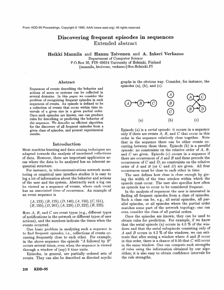
graphs in the obvious way. Consider, for instance, the
episodes (a), (b), and (c):
actions of users or systems can be collected in
several domains. In this paper we consider the
problem of recognizing frequent episodes in such
sequences of events. An episode is defined to be
a collection of events that occur within time in-
tervals of a given size in a given partial order.
Once such episodes are known, one can produce
rules for describing or predicting the behavior of
the sequence. We describe an efficient algorithm
for the discovery of all frequent episodes from a
given class of episodes, and present experimental
results.
Introduction
Most machine learning and data mining techniques are
adapted towards the analysis of unordered collections
of data. However, there are important application areas where the data to be analyzed has an inherent sequential structure.
For instance, in telecommunications network monitoring or empirical user interface studies it is easy to
log a lot of information about the behavior and actions
of the user and the system. Abstractly such a log can
be viewed as a sequence of events, where each event
has an associated time of occurrence. An example of
an event sequence is
(A, 123) (B, 125) (R140), (A, 150) (C, 151)
(B, 155), (D, 201) (A, 220), (II, 222), (B, 225).
Here A, B, and C are event types (e.g., different types
of notifications in the network or different types of user
actions), and the numbers indicate the times when the
events occurred.
One basic problem in analyzing such a sequence is
to find frequent episodes, i.e., collections of events occurring frequently close to each other. For example,
in the above sequence the episode “A followed by B”
occurs several times, even when the sequence is viewed
through a window of (say) 6 time units.
Episodes, in general, are partially ordered sets of
events. They can also be described as directed acyclic
210
KDD-95
(4
(b)
cc)
Episode (a) is a serial episode: it occurs in a sequence
only if there are events A, B, and C that occur in this
order in the sequence relatively close together. Note
that in the sequence there can be other events occurring between these three. Episode (b) is a parallel
episode: no constraints on the relative order of A, B,
and C are given. Episode (c) occurs in a sequence if
there are occurrences of A and B and these precede the
occurrences of C and D; no constraints on the relative
order of A and B (or C and 0) are given. All four
occurrences must be close to each other in time.
The user defines how close is close enough by giving the width of the time window within which the
episode must occur. The user also specifies how often
an episode has to occur to be considered frequent.
In the analysis of sequences the user is interested in
finding all frequent episodes from a class of episodes.
Such a class can be, e.g., all serial episodes, all parallel episodes, or all episodes where the partial order
matches some part of the network topology; one can
even consider the class of all partial orders.
Once the episodes are known, they can be used to
obtain rules for prediction. For example, if we know
that the serial episode (a) occurs in 4.0 % of the windows and that the serial subepisode consisting only of
A and B occurs in 4.2 % of the windows, we can estimate that after seeing a window where A and B occur
in this order, there is a chance of 0.95 that C will occur
in the same window. One can compute such strengths
of rules using the information obtained by our algorithm; it is also easy to obtain confidence intervals for
the rule strengths.
Discovery
of frequent
episodes
In this paper we
consider the following problem.
Given a class of
episodes, an input sequence of events, a window width,
and a frequency threshold, find all episodes of the class
that occur frequently enough.
We describe a general algorithm for solving this
task. The algorithm has two alternating phases: building new candidate episodes, and evaluating how often
these occur in the sequence. The efficiency of the algorithm is based on three observations:
While there are potentially a very large number of
episodes that have to be checked, the search space
can be pruned by building larger episodes from
smaller ones in a certain way. If the serial episode
ABC is frequent, with the same window width also
the serial subepisodes AB, BC, and AC are frequent. This holds in general: all subepisodes are at
least as frequent as the superepisode. Our algorithm
utilizes this observation in the opposite direction: it
is only necessary to test the occurrences of episodes
whose all subepisodes are frequent.
Episodes can be recognized efficiently by “sliding” a
window on the input sequence. Typically two adjacent windows have a lot of overlap, and are therefore
very similar to each other. We take advantage of this
similarity: after recognizing episodes in a window,
we make incremental updates in our data structures
to recognize the episodes that occur in the next window.
Recognition of a complex episode can be reduced to
the recognition of simple ones: every episode can be
seen as a recursive combination of parallel and serial
episodes. For example, the episode (c) above is a
serial combination of two episodes: (d.l), a parallel
episode consisting of A and B, and (d.2)) a parallel
episode consisting of C and D:
Related
work
For an excellent survey on patterns in
sequential data, see (Laird 1993). Wang et al. consider
the problem of discovering patterns from a number of
input sequences. Their algorithm finds patterns that
are similar to serial episodes, with respect to given minimum length, edit distance, and frequency threshold.
They also consider probabilistic pruning of patterns by
using sampling (Wang et al. 1994).
The idea of building candidate patterns from smaller
ones has been profitably used in the discovery of association rules (Mannila, Toivonen, & Verkamo 1994;
Agrawal & Srikant 1994; Agrawal et al. 1995), and
occurs also in other contexts (e.g. (Klijsgen 1995;
Wang et al. 1994)).
Taking advantage of the slowly changing contents
of the group of recent events in the recognition phase
has been studied under different fields. Within AI,
a similar problem in spirit is the many pattern/many
object pattern match problem in production system interpreters (see e.g. (Forgy 1982)). In active databases
a related problem is the efficient detection of trigger
events (see e.g. (Gehani, Jagadish, & Shmueli 1992)).
Also, comparable strategies using a sliding window
have been used e.g. to study locality of reference in
virtual memory (Denning 1968).
The methods for matching sets of episodes against
a sequence have some similarities to the algorithms
used in string matching (see (Aho 1990) for a survey).
Similarly, the work on learning regular languages from
strings has some similarities to our work. However, in
string matching or learning regular languages one typically is interested in finding substrings where there
may not be interleaved events within an occurrence of
an episode.
Formulation
Event
sequences
Given a class Ec of elementary
event types, an event is a pair (e, t), where e E Ec
and t is an integer. An event sequence S is a triple
(Z-‘,‘,,Ts, S), where TS is the starting time, Ts is the
closing time, and S is an ordered sequence of events,
i.e.,
(d-1)
(d-2)
The occurrence of an episode in a window can be
tested by using this structure and specialized methods for the recognition of parallel and serial episodes.
To see whether episode (c) occurs, we check (using
the method for serial episodes) whether (d.1) and
(d.2) occur in this order; to check the occurrence
of (d.1) we use the method for parallel episodes to
verify whether A and B occur.
We have implemented our method and used it in
the analysis of telecommunication network alarm data.
The discovered episodes have been considered useful by
domain experts.
where ei E Ec and Ts 5 ti < Ts for all i = 1, . . . , n,
andti<ti+iforalli=l,...,n-1.
A window on event sequence S = (Ts, TS, S) is
an event sequence W = (Tw , TW, W), where TS 5
Tw , TW 5 Ts, and W consists of those pairs (ei, ti)
from S where Tw 5 ti < TW. The width of the win= TW - Tw. Given an event sedow W is width(W)
quence S and an integer w, we denote by aw(S, w) the
set of all windows W on S such that width(W)
= w.
There are TS - TS - w + 1 such windows. (Also other
windowing strategies can be used, e.g., only windows
starting every w’ time units for some w’ could be considered, or windows starting from every event.)
Mannila
211
Episodes
An (elementary) episode ‘p = (V, 5, g) is a
set of nodes V, a partial order 5 on V, and a mapping
g : V + Ec associating each node with an event type.
The interpretation of an episode is that the events in
g(V) have to occur in the order described by 5.
We generalize this definition to allow for recursive
decomposition and recognition of episodes. A composite episode is an episode ‘p = (V, 5, g) such that the
mapping g is a mapping V --+ E, where the set of
event types E = Es U C, and C is the set of all composite episodes. For example, the decomposition (d) of
episode (c) above is a composite episode consisting of
two episodes; both these are composite (actually also
elementary) episodes consisting of two nodes in parallel.
The episode cp is parallel if the partial order relation
5 is trivial (i.e., II: $ y for all x: # y). The episode ‘p is
serial if the partial order relation 5 is a total order.
The crucial observation is that any elementary
episode can be equivalently described as a composite episode built recursively from parallel and serial (composite) episodes. Writing s(‘pi , . . . , cpn) and
P(Pl,
* - * , cpn) for the serial and parallel episodes consisting of episodes ‘pr , . . . , (Pi, we can write the episode
(c) above as s(p(A, B),p(C, D)).’
An episode ‘p’ = (V’, L’, g’) is a subepisode of cp =
(V, L,g), ‘p’ < cp, if V’ C V, for all v E V’, g’(v) =
g(v), and for all v, w E V’ with v 5’ w also v 5 w. An
episode ‘pi is an immediate subepisode of (p, ‘p’ <O ‘p, if
‘p’ < cp and there is no episode p” such that ‘p’ < p” <
‘p. An episode ‘p is a superepisode of ‘p’ if ‘p’ < (p, and
immediate superepisode if cp’<O cp. A class of episodes
C is closed, if for each episode ‘p in C all subepisodes
‘p’ < p are in C as well.
Frequent
episodes
An elementary
(V, 5, g) occurs in an event sequence
S=
episode P’
(Ts,TS,((el,tl),(e2,t2),...,(en,tn))),
if there exists an injective mapping h : V -+ { 1, . . . , n}
such that g(v) = ehcU) for all v E V, and for all
v, w E V with v < w, h(v) < h(w). This definition
can be generalized for composite episodes; we need
the generalization only for serial and parallel composite episodes. A parallel episode cp = (V, 5, g) occurs
in an event sequence S if all episodes in g(V) occur disjointly in S. A serial episode ‘p = (V, 5, g)
occurs in an event sequence S if there exist mappings hl, h2 : V -+ { 1, . . . , n} such that for all v E
V the subepisode g(v) occurs in the event sequence
(thl(v),th2(v) + 1, ((ehl(v),th,(v)), . . -, (ehz(v),th2(v))))
and for all v, ‘10E V with v 5 w we have h2(v) < hi(w).
1It is sometimes necessary to duplicate an event node
to obtain this decomposition; note the similarity to seriesparallel graphs. Consider, for instance, the partial order
A 2 C, B 5 C, B 2 D, where either node B or C must be
duplicated.
212
KDD-95
1.
Cl := {{e} 1 e E &I};
2.
3.
i:=l;
while
4.
5.
6.
7.
8.
Ci # 0 do
recognition: read the sequence S, and
let Li be the frequent elements of Ci
with respect to min-fr;
building: compute Ci+i c C from Li;
i := i+ 1;
od;
for
all
i,
OUtpUt
Li;
Figure 1: Main algorithm.
If an episode ‘p occurs in S, we write S 1 cp. The
of ‘p in the set aw(S, w) of all windows on S
of size w is
frequency
fr(ro, s, 4
=
I-w
E aww4
I IQ I= dl
I~W , 41
*
Given a threshold mixfr
for the frequency, a given
episode ‘p is frequent if fr(p, S, w) 2 min-fr.
If ‘p is
frequent then all its subepisodes are frequent.
The problem is now the following. Given a sequence
S, a closed class C of episodes, a window width w, and
a frequency threshold mixfr, find all frequent episodes
from S.
Algorithm
In Figure 1 we give an algorithm for finding all frequent
episodes ‘p E C in the given event sequence S, given a
closed class C of episodes and a frequency threshold
min-fr.
The algorithm works iteratively, alternating between
building and recognition phases. First, in the building
phase of an iteration i, a collection Ci of new candidate
episodes of i elementary events is built, using the information available from smaller frequent episodes. Then,
these candidate episodes are recognized in the event sequence and their frequencies are computed. The collection Li consists of frequent episodes in Ci. In the next
iteration i+ 1, candidate episodes in Ci+i are built using the information about the frequent episodes in Li.
The algorithm starts by constructing Ci to contain all
episodes consisting of single elementary events. In the
end, the frequent episodes in Li for all i are output.
Building
new
episodes
Remember that all subepisodes ‘p’ of any frequent
episode ‘p are also frequent.
That is actually the
specification of candidate episodes: in each iteration,
candidates are all those episodes of size i whose all
subepisodes are frequent.
A method to compute the candidate collection Ci is
to first generate episodes ‘p of size i, and then to test
that all immediate subepisodes ‘p’ <c ‘p are in Li-1
(see (Mannila, Toivonen, & Verkamo 1994; Agrawal &
Srikant 1994; Agrawal et al. 1995) for similar ideas).
The generation phase can be implemented efficiently
e.g. by taking pairs of episodes from Li-1 that overlap
in i - 2 nodes.
Recognizing
episodes in sequences
Episodes are recognized in sequences in an incremental
fashion. Two adjacent windows Wi = (Ti, Ti + u), Wi)
and Wi+r = (z + 1, x + w + 1, Wi+l) are typically
very similar to each other. We take advantage of this:
after recognizing episodes in Wi, we make incremental
updates in our data structures to achieve the shift of
the window to obtain Wi+r.
Remember that any elementary episode can be
viewed as a composite episode consisting of only (composite) parallel and serial episodes. In the recognition of episodes in sequences, we recursively decompose elementary episodes to parallel and serial composite episodes. To check whether a parallel episode
occurs, we apply the method below
‘p=P(Pl>...,%)
for parallel episodes; to check whether a serial episode
= s(‘p1 . . cpn) occurs, we apply the method below
Er serial ‘episbdes.2
Parallel
episodes
For simplicity, we will consider
parallel episodes ‘p = (V, 2, g) where the mapping g is
an injection, i.e. there are no two events of the same
type in an episode.
For each such candidate parallel episode ‘p we maintain a counter cp. count that indicates how many events
’ of ‘p are present in the window. When p.count becomes equal to ]cpl (indicating that ‘p is entirely included in the window) we save the index of the window
in p. inwindow.
When p.count decreases again (indicating that ‘p is no longer entirely in the window) we
increase the field p.occur by the number of windows
where ‘p remained entirely in the window.
To carry this out efficiently, the collection of candidate episodes is organized so that for each event e E E
the episodes containing e are linked together to a list
contains(e).
When the window is shifted and the set of
events in the window changes, the corresponding lists
are traversed and the counters of the episodes updated.
The requirement that the mapping g of a parallel
episode ‘p = (V, 5, g) has to be an injection can be
easily removed, allowing multisets to be presented.
Serial candidate episodes are recogSerial episodes
nized by using state automata that accept the candi2An interesting alternative approach to the recognition,
in which decomposition is not necessary, is to use inverse
structures. For each frequent episode cp’E Li we save the
indexes presenting the windows W for which W j= cp’.
Then, in the recognition phase, for a candidate episode
43E C;+l we can compute {W 1 W + P} = n{wl 1 W ’ +
‘p’ and y’ <O cp}. This holds for all but serial episodes, for
which some additional information is needed (Mannila &
Toivonen 1995; Toivonen 1995).
date episodes and ignore all other input. We initialize
a new instance of the automaton for a serial episode (p
every time the first event of ‘p comes into the window;
the automaton is removed when the same event leaves
the window. When an automaton for ‘p reaches its accepting state (indicating that ‘p is entirely included in
the window), and if there are no other automata for
‘p in the accepting state already, we save the index of
the window in cp.inwindow.
When an automaton in
accepting state is removed, and if there are no other
automata for ‘p in the accepting state (indicating that
cp is no longer entirely in the window) we increase the
field p.occur by the number of windows where ‘p remained entirely in the window.
Note that it is useless to have multiple automata
that are in the same state. It suffices to maintain the
one that reached the state last since it will be also removed last. There are thus at most 1~1 automata for
an episode ‘p. For each automata we need to know
the window index at which the automata was initialized. We represent all the automata for cp with two
arrays of size 191: one represents ‘p itself and contains
its events, the other array contains the window indices
of the automata.
To access and traverse the automata efficiently they
are organized in the following way. For each event type
e E E, the automata that accept e are linked together
to a list waits(e). When an event (e, t) enters the window during a shift, the list waits(e) is traversed and
a transition is performed in each automaton.
If an
automaton reaches a common state with another automaton, the older one is removed (i.e., overwritten).
For each event (e, t ) in the window, the automata initialized at t are linked to a list begins&(t).
When the
event is removed from the window all automata on the
list begin&(t)
are removed.3
Analysis
of time complexity
For simplicity, suppose that the candidate episodes ‘p are all of the same
size, that the class of event types E is fixed, and assume
that exactly one event takes place every time unit. Denote by m the length of the event sequence; there and
thus m - w + 1 windows, i.e., O(m).
For parallel episodes, consider w successive shifts of
one time unit. During such sequence of shifts, each of
the k candidate episodes ‘p can undergo at most 2((pl
changes: any event of an episode ‘p can be dropped out
or taken into the window at most once. This is due to
the fact that any event taken in cannot be dropped out
during the next w time units. Supposing the class of
event types E is fixed, finding the change in the set of
events during a shift of the window takes constant time.
3An obvious practical improvement to the approach
above is to combine similar prefixes of episodes and avoid
An alternative apmaintaining redundant information.
proach altogether would be to handle serial episodes basically like parallel episodes, and to check the correct ordering only when all events are in the window.
Mannila
213
w s)
Serial episodes
time (s)
16
31
ClLij
10
20
40
60
80
31
57
87
145
245
100
120
359
63
117
186
271
372
478
Parallel episodes
XjL,l
time (s)
lb
8
17
9
33
56
95
139
189
0.05
0.008
0.004
0.002
21
1 0.001
Reading the input takes time m. The total time complexity is thus O(FklpI
+ m). For a trivial nonincremental method where the sequence is preprocessed into
windows, the time requirement for recognizing k candidate episodes ‘p in m windows, plus the time required
to read in m windows of size w, is C3(mklpl + mw),
i.e., larger by a factor of w.
For serial episodes, the input sequence consists in
the worst case of events of only one event type, and
there is a serial episode ‘p of events of that same type.
Potentially every shift of the window results now in an
update in every prefix. There are m shifts, k episodes,
and IpI prefixes for each episode; the time to read the
input is m. The worst case time complexity is thus
O(mklp( + m). Th is is close to the complexity of the
trivial nonincremental method B(mklpl
+ mw).
In
practical situations, however, the time requirement is
considerably smaller, and we approach the savings obtained in the parallel case.
results
We have applied our methods to a telecommunications
network fault management database. The database
consists of 73679 alarms covering a time period of 50
days. We examined the sequence of alarm types; there
were 287 different types with diverse frequencies and
distributions.
The experiments have been run on a PC with
90 MHz Pentium processor and 16 MB main memory, under the Linux operating system. The sequence
of (alarm type, time) pairs resided in a flat text file.
Performance
overview
Tables 1 and 2 give an
overview of the discovery of frequent episodes in an empirical setting. In Table 1, serial and parallel episodes
have been discovered with a fixed frequency threshold
min-fr = 0.003 and a varying window width w; in Table 2, episodes have been discovered with a fixed window width w = 60 s and a varying frequency threshold
min-fr.
ClLil
d enotes the total number of frequent
episodes.
These experiments show that our approach is efficient. Running times are between 5 seconds and 8 min-
KDD-95
1
62
Parallel episodes
ClLil
time (s)
0
5
1
5
19
14
30
60
150
100
40
407
357
490 1
93
185
15
22
22 ]
22
Table 2: Characteristics of runs with a fixed window width w = 60 s and a varying frequency threshold min-fr.
-
214
C(L i I
0.1
14
15
21
Table 1: Characteristics of runs with a fixed frequency threshold min.-fr = 0.003 and a varying window
width w.
Experimental
Serial episodes
time (s)
0
7
1
12
min-fr
size 2
1
2
3
4
5
6
7
8
9
lo-
HS
287
lC’i[
IL;1
82369
287.0
1078.7
2 * lo7
192.4
7*10g
2 * 1ol2
6 . 1O1*
2 * 1o17
5 * 1ol9
1 * 1o22
17.4
7.1
4.7
10.1
2.9
2.1
1.7
1.4
16.0
2.1
1.7
17.4
30.1
44.6
20.0
5.3
2.9
Match
11 %
4 %
10 %
58 %
74 %
61 %
75 %
80 %
83 %
92 %
Table 3:
Number of serial candidate and frequent episodes per iteration with frequency threshold min-fr = 0.003, averaged over window widths
w= 10,20,40,60,80,100,
and 120 s. HS is the size of
the hypothesis space; ‘match’ is the fraction ILil/lCil.
utes, in which time hundreds of frequent episodes could
be found. Relatively small changes in the parameters influence the number of episodes found, but the
method is robust in the sense that a change in one parameter does not result in the replacement of any of
the episodes found.
Quality
of candidate
generation
Table 3 presents
the number of serial candidate and frequent episodes
per iteration averaged over a number of test runs.
In the first iteration, for size i = 1, all 287 elementary events have to be checked. The larger the episodes
become, the more combinatorial
information
there exists to take advantage of. From size 4 up, over one half
of the candidates turned out to be frequent.4
recognition
Figure 2 presents the ratio of times needed for trivial vs. incremental recognition of candidate episodes. The figure shows that
Incremental
*Another possible improvement is to combine iterations
by generating candidate episodes for several iterations at
once, and thus avoid reading the input sequence so many
times. This pays off in the later iterations, where there are
otherwise only few candidates to recognize, and where the
match is good.
201
Efficiency
ratio
’
I
I
I
is efficient. We have applied the method in the analysis
of the alarm flow from a telecommunications network.
Discovered episodes have been considered useful by domain experts.
We are currently investigating the use of inverse
structures in the recognition phase of the algorithm.
The preliminary results are quite encouraging.
I
15
10
5
0
0
20
40 60 80 100 120
Window width w (s)
Figure 2: Ratio of times needed for trivial vs. incremental recognition methods for parallel (solid line) and
serial episodes (dotted line) as functions of window
width u).
500 )’
I-
012
:
-I
4
8
Relative size of database
Figure 3: Scale-up results for parallel (solid line)
and serial episodes (dotted line) with UI = 60 s and
min-fr = 0.01.
the incremental methods are faster by a factor of 1 20, approximately linearly with respect to the window
width (10 - 120). Th is matches the worst case analysis
of recognizing parallel episodes, and indicates that the
incremental recognition method is useful in practice
also for serial episodes.
Scale-up
We performed scale-up tests with 1 to 8
fold multiples of the database, i.e. sequences with 74
to 590 thousand events. Figure 3 shows that the time
requirement is linear with respect to the length of the
input sequence, as could be expected from the analysis.
Conclusions
We have presented a framework for discovering frequent episodes in sequential data. The framework consists of defining episodes as partial orders, and looking
at windows of the sequence. We described an algorithm
for finding all episodes from a given class of episodes
that are frequent enough. The algorithm was based
on the discovery of episodes by only considering an
episode when all its subepisodes are frequent, and on
incremental checking of whether an episode occurs in a
window. The implementation shows that the method
References
Agrawal, R., and Srikant, R. 1994. Fast algorithms for
mining association rules in large databases. In 20th
International
(VLDB 94).
Conference
on Very
Large
Databases
Agrawal, R.; Mannila, H.; Srikant, R.; Toivonen, H.;
and Verkamo, A. I. 1995. Fast discovery of association rules. In Fayyad, U. M.; Piatetsky-Shapiro, G.;
Smyth, P.; and Uthurusamy, R., eds., Advances in
Knowledge Discovery and Data Mining. AAAI Press.
To appear.
Aho, A. V. 1990. Algorithms for finding patterns in
strings. In van Leeuwen, J., ed., Handbook of Theoretical Computer Science, Volume A: Algorithms
Complexity.
Elsevier. 255-400.
and
Denning, P. J. 1968. The working set model of
Communications
of the ACM
program behavior.
11(5):323 - 333.
Forgy, C. L. 1982. Rete: A fast algorithm for the
many pattern/many
object pattern match problem.
Artificial
Intelligence
19117 - 37,
Gehani, N.; Jagadish, H.; and Shmueli, 0. 1992.
Event specification in an active object-oriented
database. In 1992 International
Conference on Management of Data (SIGMOD
92), 81 - 90.
Kltisgen, W. 1995. Efficient discovery of interesting
statements in databases. Journal of Intelligent Information Systems 4(1):53 - 69.
Laird, P. 1993. Identifying and using patterns in
Learning Theory, 4th
sequential data. In Algorithmic
International
Workshop, 1 - 18. Springer-Verlag.
Mannila, H., and Toivonen, H. 1995. Discovering frequent episodes in sequences using inverse structures.
Manuscript in preparation.
Mannila, H.; Toivonen, H.; and Verkamo, A. I.
1994. Efficient algorithms for discovering association
rules. In AAAI Workshop on Knowledge Discovery in
Databases (KDD 94) , 181 - 192.
Toivonen, H. 1995. Ph.D. thesis in preparation.
Wang, J. T.-L.; Chirn, G.-W.; Marr, T. G.; Shapiro,
B.; Shasha, D.; and Zhang, K. 1994. Combinatorial
pattern discovery for scientific data: Some prelimiConference on
nary results. In 1994 International
Management
of Data (SIGMOD
94), 115 - 125.
Mannila
215