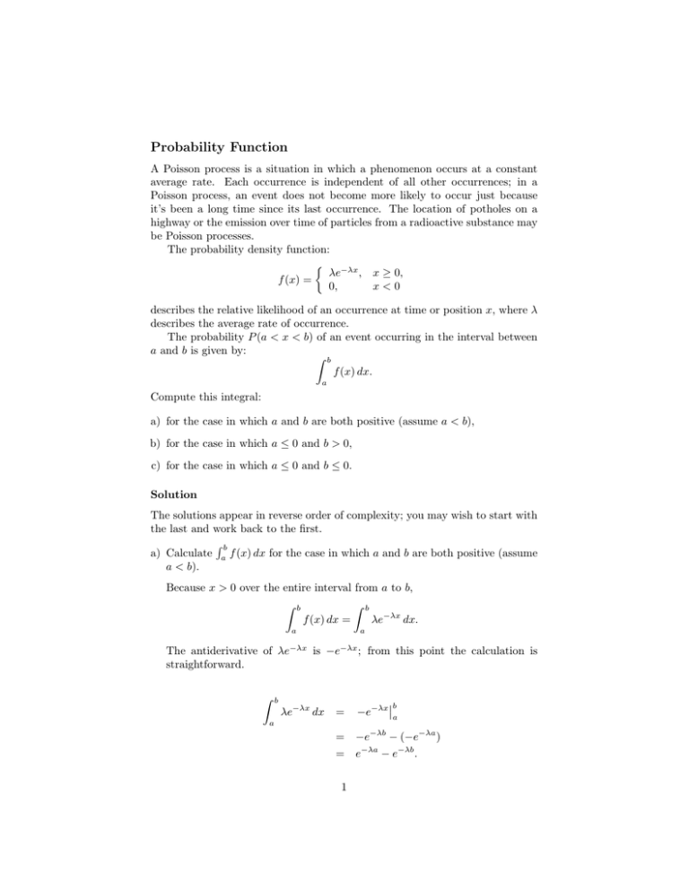
Probability Function
A Poisson process is a situation in which a phenomenon occurs at a constant
average rate. Each occurrence is independent of all other occurrences; in a
Poisson process, an event does not become more likely to occur just because
it’s been a long time since its last occurrence. The location of potholes on a
highway or the emission over time of particles from a radioactive substance may
be Poisson processes.
The probability density function:
�
λe−λx , x ≥ 0,
f (x) =
0,
x<0
describes the relative likelihood of an occurrence at time or position x, where λ
describes the average rate of occurrence.
The probability P (a < x < b) of an event occurring in the interval between
a and b is given by:
� b
f (x) dx.
a
Compute this integral:
a) for the case in which a and b are both positive (assume a < b),
b) for the case in which a ≤ 0 and b > 0,
c) for the case in which a ≤ 0 and b ≤ 0.
Solution
The solutions appear in reverse order of complexity; you may wish to start with
the last and work back to the first.
�b
a) Calculate a f (x) dx for the case in which a and b are both positive (assume
a < b).
Because x > 0 over the entire interval from a to b,
� b
� b
f (x) dx =
λe−λx dx.
a
a
The antiderivative of λe−λx is −e−λx ; from this point the calculation is
straightforward.
�
b
λe−λx dx
=
a
�b
−e−λx �a
= −e−λb − (−e−λa )
= e−λa − e−λb .
1
Given a Poisson distribution with rate parameter λ and b ≥ a > 0, the
probability of an event occurring in the interval [a, b] is e−λa − e−λb .
b) Calculate
�b
a
f (x) dx for the case in which a ≤ 0 and b > 0.
We haven’t done many examples of integration of piecewise defined func­
tions, but we can use the geometric interpretation of the definite integral to
determine what we must do.
On the interval [a, 0], f (x) = 0 so the area under that part of the graph of
f (x) is 0. On the interval [b, 0], f (x) = λe−λx . The area under the graph of
f (x) between a and b must be:
�
b
0
�
f (x) dx
=
a
�
a
f (x) dx
0
�
=
b
f (x) dx +
0+
b
λe−λx dx
0
c) Calculate
�b
a
=
�b
−e−λx �0
=
=
−e−λb − (−e−λ·0 )
1 − e−λb .
f (x) dx for the case in which a ≤ 0 and b ≤ 0.
This calculation is trivial. On the interval [a, b], f (x) = 0. The area between
the graph of f and the x-axis is 0, so:
�
b
f (x) dx = 0
a
2
when a, b ≤ 0.
MIT OpenCourseWare
http://ocw.mit.edu
18.01SC Single Variable Calculus��
Fall 2010 ��
For information about citing these materials or our Terms of Use, visit: http://ocw.mit.edu/terms.