From: KDD-97 Proceedings. Copyright © 1997, AAAI (www.aaai.org). All rights reserved.
Analysis
Comparison
and Visualization
under Imprecise
Foster
Provost
NYNEX Science and Technology
400 Westchester Avenue
White Plains, New York 10604
foster@nynexst.com
Abstract
Applications of inductive learning algorithms to realworld data mining problems have shown repeatedly
that using accuracy to compare classifiers is not adequate because the underlying assumptions rarely hold.
We present a method for the comparison of classifier
performance that is robust to imprecise class distributions and misclassification costs. The ROC convex
hull method combines techniques from ROC analysis, decision analysis and computational geometry, and
--~-I---!
--I--,- LT.-.iearned
aaapss
r;nem L50 11~.
cne ..-.,I--.,parr;iculars 01-f analyzing
classifiers. The method is efficient and incremental,
minimizes the management of classifier performance
data, and allows for clear visual comparisons and sensitivity analyses.
Introduction
When mining data with inductive methods, we often
experiment with a wide variety of learning algorithms,
using different algorithm parameters, varying output
threshold values, and using different training regimens.
Such experimentation yields a large number of classifiers to be evaluated and compared. In order to compare the performance of classifiers it is necessary to
know the conditions under which they will be used;
using accuracy alone is inadequate because class distributions and misclassification costs are rarely uniform.
Decision-theoretic principles may be used if the class
and cost distributions are known exactly. Unfortunately, on real-world problems target cost and class
distributions can rarely be specified precisely, and they
are often subject to change. For example, in fraud detection we cannot ignore either type of distribution,
nor can we assume that our distribution specifications
are static or precise. We need a method for the management and comparison of multiple classifiers that is
robust to imprecise and changing environments.
We introduce the ROC convex hull method, which
combines techniques from ROC analysis, decision analCopyright 01997, American Association for Artificial Intelligence (www.aaai.org). All rights reserved.
of Classifier Performance:
Class and Cost Distributions
Tom Fawcett
NYNEX Science and Technology
400 Westchester Avenue
White Plains, New York 10604
fawcett@nynexst.com
ysis and computational geometry. The method decouples classifier performance from specific class and cost
distributions, and may be used to specify the subset of
methods that are potentially optimal under any cost
and class distribution assumptions.
The ROC convex hull method is efficient, so it facilitates the comparison of a large number of classifiers.
It minimizes the management of classifier performance
data, because it can specify exactly those classifiers
that are potentially optimal, and it is incremental, easily incorporating new and varied classifiers.
The Inadequacy
of Accuracy
A tacit assumption in the use of classification accuracy
as an evaluation metric is that the class distribution
among examples is constant and relatively balanced. In
the real world this is rarely the case. Classifiers are
often used to sift through a large population of normal
or uninteresting entities in order to find a relatively
small number of unusual ones, for example, looking
for defrauded customers or checking an assembly line
for defective parts. Because the unusual or interesting
class is rare among the general population, the class
distribution is very skewed (Ezawa, Singh, & Norton
1996; Fawcett & Provost 1996).
As the class distribution becomes more skewed, evaluation based on accuracy breaks down. Consider a
domain where the classes appear in a 999:l ratio. A
simple rule, always classify as the maximum likelihood
class, gives a 99.9% accuracy. Presumably this is not
satisfactory if a non-trivial solution is sought. Skews of
lo2 are common in fraud detection and skews greater
than lo6 have been reported in other classifier learning
applications (Clearwater & Stern 1991).
Evaluation by classification accuracy also tacitly assumes equal error costs-that
a false positive error
is equivalent to a false negative error. In the real
world this is rarely the case, because classifications lead
to actions which have consequences, sometimes grave.
Rarely are mistakes evenly weighted in their cost. Indeed, it is hard to imagine a domain in which a learning system may be indifferent to whether it makes a
false positive or a false negative error. In such cases,
Provost
43
accuracy maximization should be replaced with cost
minimization.
The problems of unequal error costs and uneven class
distributions are related. It has been suggested that
high-cost instances can be compensated for by increasing their prevalence in an instance set (Breiman et al.
1984). Unfortunately, little work has been published
on either problem. There exist several dozen articles
(Turney 1996) in which techniques are suggested, but
little is done to evaluate and compare them (the article
of Pazzani et al. (1994) being the exception). The literature provides even less guidance in situations where
distributions are imprecise or can change.
Evaluating
and Visualizing
Performance
Classifier
To discuss classifier evaluation we use the following
terminology. Let {p,n) be the positive and negative
instance classes, and let {Y,N}
be the classifications
produced by a classifier. Let p(pJI) be the posterior
probability that instance I is positive. The true positive rate, TP, of a classifier is:
TP =PW!P)
=
positives correctly classified
> >~,
.>.
total positives
The false positive rate, FP, of a classifier is:
FP = p(YJn) M
negatives incorrectly classified
total negatives
Let c(classification, class) be a two-place error cost
function where c(Y, n) is the cost of a false positive
error and c(N, p) is the cost of a false negative error’.
If a classifier produces posterior probabilities, decision
analysis gives us a way to produce cost-sensitive classifications from the classifier (Weinstein & Fineberg
1980). Classifier error frequencies can be used to approximate probabilities (Pazzani et al. 1994). For an
instance I, the decision to emit a positive classification
is:
[l - P(PIOI .4Y,
4
< ~(~11) .c(N, PI
Regardless of whether a classifier produces probabilistic or binary classifications, its normalized cost on
a test set can be evaluated empirically as:
Cost = FP . c(Y, n) + FN . c(N, p)
Given a set of classifiers, a set of examples, and a precise cost function, most work on cost-sensitive classification uses an equation such as this to rank the classifiers according to cost and chooses the minimum. However, as discussed above, such analyses assume that the
distributions are precise and static.
Receiver Operating Characteristic (ROC) graphs
have long been used in signal detection theory to depict tradeoffs between hit rate and false alarm rate
‘Error costs include benefits not realized.
44
KDD-97
1
M
0.1
False Positge rate0.8
Figure 1: An ROC graph of four classifiers
(Egan 1975). ROC analysis has been extended for use
in visualizing and analyzing the behavior of diagnostic
systems (Swets 1988), and is used for visualization in
medicine (Beck & Schultz 1986).
We will use the term ROC space to denote the classifier performance space used for visualization in ROC
analysis. On an ROC graph, TP is plotted on the Y
1-s
axis and- f+
Y is piotted on the x axis. ‘These statistics
vary together as a threshold on a classifier’s continuous
output is varied between its extremes, and the resulting curve is called the ROC curve. An ROC curve
illustrates the error tradeoffs available with a given
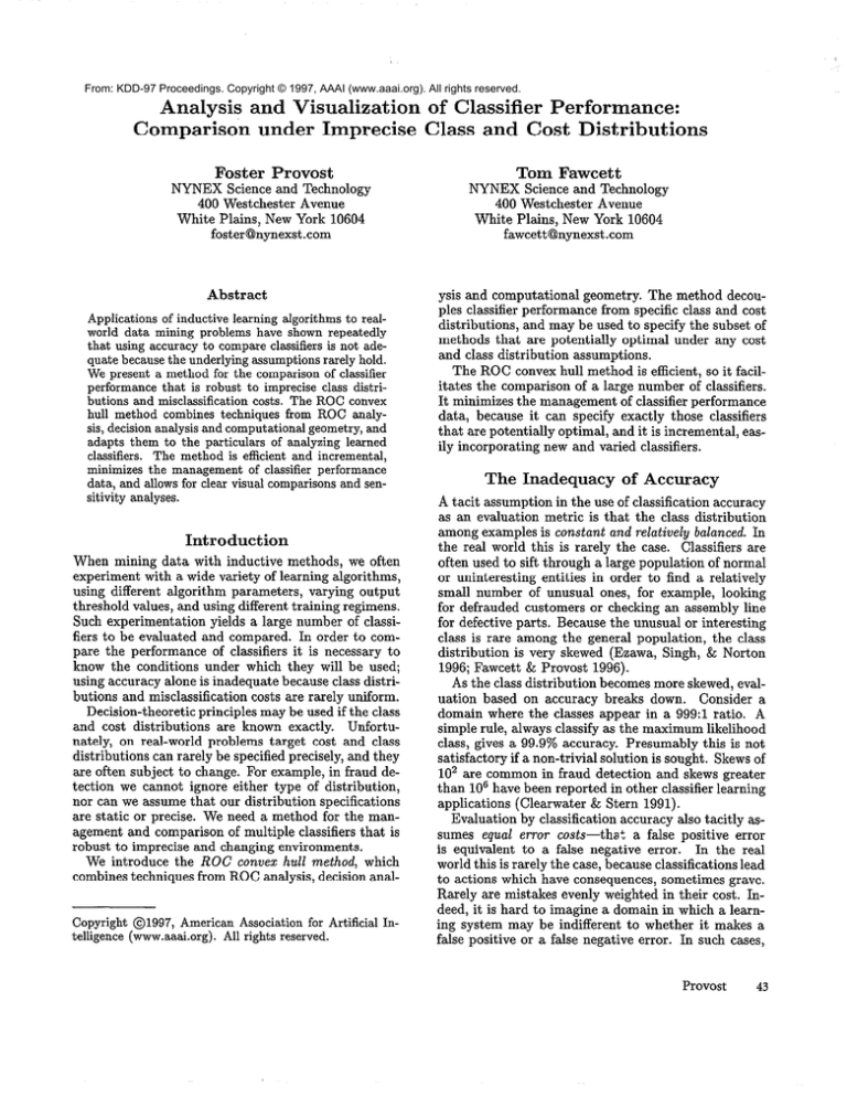
classifier. Figure 1 shows a plot of the performance
of four classifiers, A through D, typical of what we see
in the creation of alarms for fraud detection (Fawcett
& Provost 1996).
For orientation, several points on an ROC graph
should be noted. The lower left point (0,O) represents
the strategy of never alarming, the upper right point
(1,1) represents the strategy of always alarming, the
point (0,l) represents perfect classification, and the
line y = x (not shown) represents the strategy of randomly guessing the class. Informally, one point in ROC
space is better than another if it is to the northwest
(TP is higher, FP is lower, or both). An ROC graph
allows an informal visual comparison of a set of classifiers. In Figure 1, curve A is better than curve D
because it dominates in all points.
ROC graphs illustrate the behavior of a classifier
without regard to class distribution or error cost, and
so they decouple classification performance from these
factors. Unfortunately, while an ROC graph is a valuable visualization technique, ROC analysis does a poor
job of aiding the choice of classifiers. Only when one
ciassifier cieariy dominates another over the entire performance space can it be declared better. Consider the
classifiers shown in Figure 1. Which is best? The answer depends upon the performance requirements, i.e.,
the error costs and class distributions in effect when the
classifiers are to be used.
Some researchers advocate choosing the classifier
that maximizes the product (1 - FP) - TP. Geometrically, this corresponds to fitting rectangles under every ROC curve and choosing the rectangle of greatest
area- This and other approaches that calculate average
performance over the entire performance space (Swets
1988; Beck & Schultz 1986) may be appropriate if costs
and class distributions are completely unknown and a
single classifier must be chosen to handle any situation. However, they will choose a suboptimal classifier
in many situations.
The
ROC
Convex
Hull
Method
In this section we combine decision analysis with ROC
analysis and adapt them for comparing the performance of a set of learned classifiers. The method is
based on three high-level principles. First, the ROC
space is used to separate classification performance
from class and cost distribution information.
Second, decision-analytic information is projected onto
the ROC space. Third, we use the convex hull in ROC
space to identify the subset of methods that are potentially optimal.
Iso-performance
0.2
0.4
0.6
0.8
I.0
False Positive rate
Figure 2: The ROC convex hull identifies potentially
optimal classifiers.
lines
By separating classification performance from class
and cost distribution assumptions, the decision goal
can be projected onto ROC space for a neat visualization. Formally, let the prior probability of a positive
example be p(p), so the prior probability of a negative
example is p(n) = 1 -p(p).
Costs of false positive and
false negative errors are given by c(Y, n) and c(N, p),
respectively. The expected cost of a classification by
the classifier represented by a point (TP,FP) in ROC
space is:
P(P) * (1 -TP).c(N,p)
+ dn).FP.c(Y,n)
Therefore, two points, (TPl,FPl)
have the same performance if
and (TPz,FPz),
TP2 - TP1
dn)4Y,
4
FP2 - FP1 = P(P)~>P)
This equation defines the slope of an iso-performance
line, i.e., all classifiers corresponding to points on the
line have the same expected cost. Each set of class and
cost distributions defines a family of iso-performance
lines. Lines “more northwest”-having
a larger TPintercept-are
better because they correspond to classifiers with lower expected cost.
The ROC convex hull
Because in most real-world cases the target distributions are not known precisely, it is valuable to be able
to identify what subset of classifiers is potentially optimal. Each possible set of distributions defines a family of iso-performance lines, and for a given family,
the optimal methods are those that lie on the “mostnorthwest” iso-performance line. Thus, a classifier is
0.2
0.4
0.6
0.8
1.”
False Positive rate
Figure 3: Lines Q and p show the optimal
under different sets of conditions.
classifier
potentially optimal if and only if it lies on the northwest boundary (i.e., above the line y = x) of the convex
hull (Barber, Dobkin, & Huhdanpaa 1993) of the set
of points in ROC space. Space limitations prohibit a
formal proof, but one can see that if a point lies on the
conwex hull, then there exists a line through that point
such that no other line with the same slope through
any other point has a larger TP-intercept,
and thus
the classifier represented by the point is optimal under
any distribution assumptions corresponding the that
slope. If a point does not lie on the convex hull, then
for any family of iso-performance lines there is another
point that lies on an iso-performance line with the same
slope but larger TP-intercept, and thus the classifier
cannot be optimal.
We call the convex hull of the set of points in ROC
space the ROC convex hull of the corresponding set
of classifiers. Figure 2 shows the curves of Figure 1
with the ROC convex hull drawn (CH, the border between the shaded and unshaded areas). D is clearly not
optimal. Surprisingly, B can never be optimal either
because none of the points of its ROC curve lies on the
convex hull. We can also remove from consideration
Provost
45
any points of A and C that do not lie on the hull.
Consider these classifiers under two distribution scenarios. In each, negative examples outnumber positives by 1O:l. In scenario AA, false positive and false
negative errors have equal cost. In scenario a, a false
negative is 100 times as expensive as a false positive
(e.g., missing a case of fraud is much worse than a
false alarm). Each scenario defines a family of isoperformance lines. The lines corresponding to scenario
A have slope 10; those for B have slope &. Figure 3
shows the convex hull and two iso-performance lines,
cx and p. Line a is the “best” line with slope 10 that
intersects the convex hull; line p is the best line with
slope h that intersects the convex hull. Each line identifies the optimal classifier under the given distribution.
Generating
the ROC
Convex
Hull
We call the comparison of classifier performance based
on the ROC convex hull and iso-performance lines the
ROC convex hull method.
1. For each classifier, plot TP and FP in ROC space.
For continuous-output classifiers, vary a threshold
over the output range and plot the ROC curve.
9 l7:ns-l
Y.
I lll.2
tha
PAIIIIPV
IJIIC lr”Il.YOn
hnll
LlUll
nf thn
“L
“I.b
nnt “Inf
ObU
nn;ntc
p”IIIYu
,.m-.vrxnmtLtiyrulGuu-
ing the predictive behavior of all classifiers of interest. For n classifiers this can be done in O(n log(n))
time by the QuickHull algorithm (Barber, Dobkin,
& Huhdanpaa 1993).
3. For each set of class and cost distributions of interest, find the slope (or range of slopes) of the corresponding iso-performance lines.
4. For each set of class and cost distributions, the optimal classifier will be the point on the convex hull
that intersects the iso-performance line with largest
TP-intercept.
Ranges of slopes specify hull segments.
Using
the ROC
Convex
Hull
Figures 2 and 3 demonstrate how the subset of classifiers that are potentially optimal can be identified
and how classifiers can be compared under different
cost and class distributions. We now demonstrate additional benefits of thq method.
Comparing
a variety
of classifiers
The ROC convex hull method accommodates both binary and continuous classifiers. Binary classifiers are
represented by individual points in ROC space. Continuous classifiers produce numeric outputs to which
threshoids can be appiied, yieiding a series of (FP, TP)
pairs comprising an ROC curve. Each point may or
may not contribute to the ROC convex hull. Figure 4
depicts the binary classifiers E, F and G added to the
previous hull. E may be optimal under some circumstances because it extents the convex hull. Classifiers
F and G will never be because they do not extend it.
46
KDD-97
0.2
0.4
0.6
0.8
1.0
False Positive rate
Figure 4: Classifier E may be optimal because it extends the ROC convex hull. F and G cannot because
they do not.
New classifiers can be added incrementally to an
ROC convex hull analysis, as demonstrated above with
the addition of classifiers E,F, and G. Each new classifier either extends the existing hull or does not. In
the former case the hull must be updated accordingly,
but in the iatter case the new classifier can be ignored.
Therefore, the method does not require saving every
classifier (or saving statistics on every classifier) for reanalysis under different conditions-only
those points
on the convex hull. No other classifiers can ever be optimal, so they need not be saved. Every classifier that
does lie on the convex hull must be saved.
Changing
distributions
and costs
Class and cost distributions that change over time
necessitate the reevaluation of classifier choice. In
fraud detection, costs change based on workforce and
reimbursement issues; the amount of fraud changes
monthly. With the ROC convex hull method, comparing under a new distribution involves only calculating the slope(s) of the corresponding iso-performance
lines and intersecting them with the hull, as shown in
Figure 3.
The ROC convex hull method scales gracefully to
any degree of precision in specifying the cost and class
distributions. If nothing is known about a distribution,
the ROC convex hull shows all classifiers that may be
optimal under any conditions. Figure 2 showed that,
given classifiers A, B, C and D of Figure 1, only A and
C can ever be optimal.
--_. _
With compiete information, the method identifies
the optimal classifier(s). In Figure 3 we saw that classifier A (with a particular threshold value) is optimal
under scenario A and classifier C is optimal under scenario Z?. Next we will see that with less precise information, the ROC convex hull can show the set of
possibly optimal classifiers.
Sensitivity
analysis
Imprecise distribution information defines a range of
slopes for iso-performance lines. This range of slopes
intersects a segment of the ROC convex hull, which
facilitates sensitivity analysis. For example, if the segment defined by a range of slopes corresponds to a
single point in ROC space or a small threshold range
for a single classifier, then there is no sensitivity to the
distribution assumptions in question. Consider a scenario similar to A and a in that negative examples are
10 times as prevalent as positive ones. In this scenario,
the cost of dealing with a false alarm is between $5 and
$10, and the cost of missing a positive example is between $500 and $1000. This defines a range of slopes
for iso-performance lines: $ _< m 5 5. Figure 5a
depicts this range of slopes and the corresponding segment of the ROC convex hull. The figure shows that
the choice of classifier is insensitive to changes within
this range (and tuning of the classifier’s threshold will
be relatively small). Figure 5b depicts a scenario with
a wider range of slopes: i 5 m < 2. The figure shows
that under this scenario the choice of classifier is very
sensitive to the distribution.
Classifiers A, C and E
each are optimal for some subrange.
A
is.
_- narticularlv
r..-IT---.lmwJ intsrestinp
----1---LJ--- o nueqtinn
x--L1---- in
__.anv
_.-.~ damain
-- ---..___A>
When is a “do nothing” strategy better than any of my
available classifiers? Consider Figure 5c. The point
(0,O) corresponds to doing nothing, i.e., issuing negative classifications regardless of input. Any set of cost
and class distribution assumptions for which the best
hull-intersecting
iso-performance line passes through
the origin (e.g., line Q) defines a scenario where this
null strategy is optimal. In the example of Figure 5c,
the range of scenarios is small for which the null strategy is optimal; the slopes of the lines quantify the
range.
Limit at ions and Implications
In this paper, we have simplified by assuming there are
only two classes and that costs do not vary within a
given type of error. The first assumption is essential
to the use of a two dimensional graph; the second assumption is essential to the creation of iso-performance
lines. Furthermore, the method is based upon the maximization of expected value as the decision goal. Other
decision goals are possible (Egan 1975). For example,
the Neyman-Pearson observer strategy tries to maximize the hit rate for a fixed false-alarm rate. In our
framework, a Neyman-Pearson observer would find the
vertical line corresponding to the given FP rate, and
intersect it with a “non-decreasing” hull, rather than
Al-^^- __^__
L...,,
,---I -IIIUYB
-^--^ IAL
~~-L~I1Idle c;“.lI”tx
m.l11\anu
Itxb L~-‘
II”~-l‘
“IIbally, IP---2Ll-\
,I y”sal”la,.
Also, methods such as these should consider statistical tests for comparing performance curves, so that the
user has confidence that differences in performance are
significant.
The tradeoff between TP and FP rates is similar to the tradeoff between precision and recall, com-
monly used in Information Retrieval (Bloedorn, Mani,
& MacMillan 1996). However, precision and recall do
not take into account the relative size of the population of “uninteresting” entities, which is necessary to
deal with changing class distributions.2
Existing cost-sensitive learning methods are brittle
with respect to imprecise or changing distributions.
These methods can be categorized into four categories:
(i) the use of cost distribution in building a classifier,
e.g., for choosing splits in a decision tree or for building rule sets (Breiman et al. 1984; Pazzani et al. 1994;
Provost & Buchanan 1992); (ii) the use of the cost
distribution in post-processing the classifier, e.g., for
pruning a decision tree (Breiman et al. 1984; Pazzani
et al. 1994), for finding rule subsets (Catlett 1995;
Provost & Buchanan 1995), or for setting an output
threshold; (iii) estimate the probability distribution
and use decision-analytic combination (Pazzani et al.
1994; Catlett 1995; Duda & Hart 1973); and (iv) search
for a bias with which a good classifier can be learned
(Turney 1995; Provost & Buchanan 1995). Of these,
only probability estimation methods (iii) can handle
changes in cost (or class) distribution without modifying the classifier. However, no single method dominates all others, so the ROC convex hull is still needed
for comparison. As future work, we propose the development of methods that search explicitly for classifiers
that extend the ROC convex hull.
Conclusion
The ROC convex hull method is a robust, efficient
solution to the problem of comparing multiple classifiers in imprecise and changing environments.
It is
intuitive, can compare classifiers both in general and
under specific distribution assumptions, and provides
crisp visualizations. It minimizes the management of
classifier performance data, by selecting exactly those
classifiers that are potentially optimal; thus, only these
data need to be saved in preparation for changing conditions. Moreover, due to its incremental nature, new
classifiers can be incorporated easily, e.g., when trying
a new parameter setting.
It has been noted many times that costs and class
distributions are difficult to specify precisely. Classifier learning research should explore flexible systems
that perform well under a range of conditions, perhaps
for part of ROC space. We hope that our method for
analysis of classifiers can help free researchers from the
need to have precise class and cost distribution information.
2Thanks to Peter Turney for an enlightening
on the application of this approach to IR.
discussion
Provost
47
0.2
0.4
0.6
0.8
False Positive rate
0.z
0.4
0.6
0.8
False Positive rate
(4
(b)
0
0.2
0.4
0.6
0.8
False Positive rate
(4
Figure 5: Sensitivity analysis using the ROC convex hull: (a) low sensitivity (only C can be optimal),
sensitivity (A, E, or C can be optimal), (c) doing nothing is the optimal strategy
References
Barber, C.; Dobkin, D.; and Huhdanpaa, H.
1993. The quickhull algorithm for convex hull.
Technical Report GCG53, University
of Minnesota. Available from ftp://geom.umn.edu/pub/
software/qhull.tar.Z.
Beck, J. R., and Schultz, E. K. 1986. The use of ROC
curves in test performance evaluation. Arch Path01
Lab Med 110:13-20.
Bloedorn, E.; Mani, I.; and MacMillan, T. 1996. Machine learning of user profiles: Representational issues. In Proceedings of Thirteenth National Conference on Artijicial Intelligence, 433-438. Menlo Park,
CA: AAAI Press.
Breiman, L.; Friedman, J.; Olshen, R.; and Stone, C.
1984. Classification and regression trees. Belmont,
CA: Wadsworth International Group.
Catlett, J. 1995. Tailoring rulesets to misclassificatioin costs. In Proceedings of the 1995 Conference on
AI and Statistics, 88-94.
Clearwater, S., and Stern, E. 1991. A rule-learning
program in high energy physics event classification.
Comp Physics Comm 67:159-182.
Draper, B.; Brodley, C.; and Utgoff, P. 1994. Goaldirected classification using linear machine decision
trees. IEEE Transactions on Pattern Analysis and
Machine Intelligence 16(9):888-893.
Duda, R. O., and Hart, P. E. 1973. Pattern Classij%
cation and Scene Analysis. New York: John W iley.
Egan, J. P. 1975. Signal Detection Theory and ROC
Analysis. Series in Cognitition and Perception. New
York: Academic Press.
Ezawa, K.; Singh, M.; and Norton, S. 1996. Learning
goal oriented bayesian networks for telecommunica-
48
KDD-97
(b) high
tions risk management. In Proceedings of IMLC-96,
139-147. San Francisco, CA: Morgan Kaufmann.
Fawcett, T., and Provost, F. 1996. Combining data
mining and machine learning for effective user profiling. In Proceedings of KDD-96, 8-13. Menlo Park,
CA: AAAI Press.
Pazzani, M.; Merz, C.; Murphy, P.; Ali, K.; Hume, T.;
and Brunk, C. 1994. Reducing misclassification costs.
In Proc. 11th International Conference on Machine
Learning, 217-225. Morgan Kaufmann.
Provost, F., and Buchanan, B. 1992. Inductive policy.
In Proceedings of AAAI-92, 255-261. Menlo Park,
CA: AAAI Press.
Provost, F., and Buchanan, B. 1995. Inductive policy:
The pragmatics of bias selection. Machine Learning
20:35-61.
Saitta, L.; Giordana, A.; and Neri, F. 1995. What is
the “real-world”? In IMLC-95 Workshop on Applying
Machine Learning in Practice (Tech Rept. AIC-95023 Naval Research Lab), 34-40.
Swets, J. 1988. Measuring the accuracy of diagnostic
systems. Science 240:1285-1293.
Turney, P. 1995. Cost-sensitive classification: Empirical evaluation of a hybrid genetic decision tree induction algorithm. JAIR 2:369-409.
Turney, P.
1996. Cost sensitive learning bibliography. http://ai.iit.nrc.ca/bibl.iographies/
cost-sensitive.html.
Weinstein, M. C., and Fineberg, H. V. 1980. Clinical
Decision Analysis. Philadelphi, PA: W . B. Saunders
Company.