From: KDD-96 Proceedings. Copyright © 1996, AAAI (www.aaai.org). All rights reserved.
Efficient
Implementation
of Data
Jeffrey
Cubes
Via Materialized
Views
”
D. Ullman
Department of Computer Science
Stanford University
Stanford CA 94305
ullman6cs. stanford.edu
http://db.stanford.edu/‘ullman
Abstract
Data cubes are specialized database management systems designed to support multidimensional
data for
such purposes as decision support and data mining. For
a given mix of queries, we can optimize the implementation of a data cube by materializing some projections
of the cube. A greedy approach turns out to be very
effective; it is both polynomial-time as a function of the
number of possible views to materialize and guaranteed
to come close to the optimum choice of views. The work
reported here is a summary of results appearing in the
following two papers:
V. Harinarayan, A. Rajaraman, and J. D. Ullman,
To appear
“Implementing
data cubes efficiently.”
in 1996 SIGMOD. An extended version is availas
able by anonymous ftp from db. stanford.edu
pub/harinarayan/i995/cube.ps.
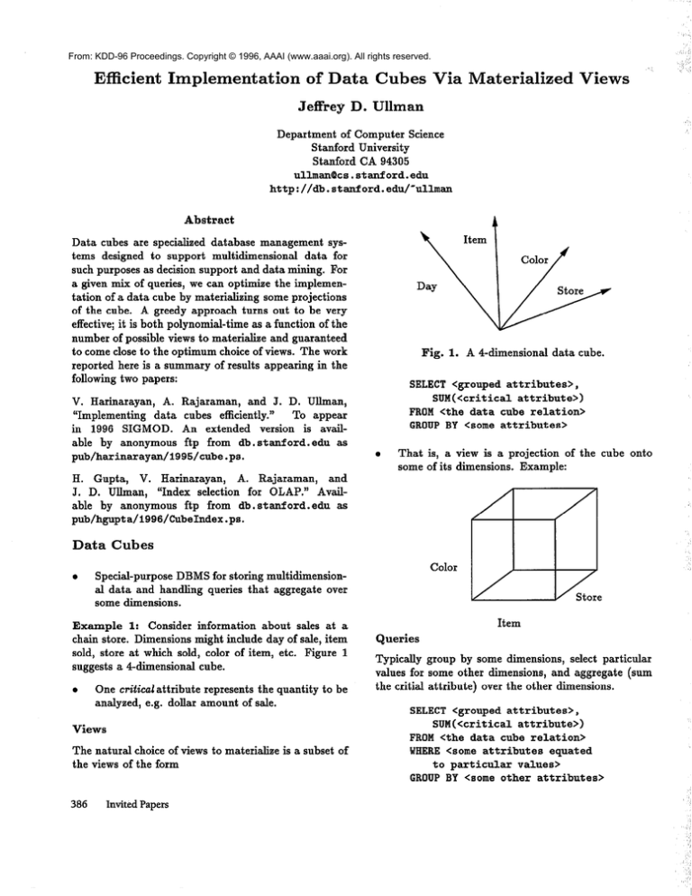
Fig. 1. A 4-dimensional
data cube.
SELECT <grouped attributes>,
SUM(tcritica1
attribute>)
FROM <the data cube relation>
GROUPBY <some attributes>
a
That is, a view is a projection of the cube onto
some of its dimensions. Example:
H. Gupta, V. Harinarayan,
A. Rajaraman,
and
J. D. Ullman, “Index selection for OLAP.” Available by anonymous ftp from db. stanford.edu
as
pub/hgupta/i996/CubeIndex.ps.
Data
l
Cubes
Example
1: Consider information about sales at a
chain store. Dimensions might include day of sale, item
sold, store at which sold, color of item, etc. Figure 1
suggests a 4dimensional cube.
l
One critical attribute represents the quantity to be
analyzed, e.g. dollar amount of sale.
Views
The natural choice of views to materialize is a subset of
the views of the form
386
Color
Special-purpose DBMS for storing multidimensional data and handling queries that aggregate over
some dimensions.
Invited Papers
Item
Queries
Typically group by some dimensions, select particular
values for some other dimensions, and aggregate (sum
the critial attribute) over the other dimensions.
SELECT <grouped attributes>,
SUM(<critical
attribute>)
FROM <the data cube relation>
WHERE<some attributes
equated
to particular
values>
GROUPBY <some other attributes>
‘(, ,;I
Want to select the 3 views that most improve the
average query cost.
l
First Choice
Second Choice
Optimum = 1
Third Choice
b 50 x 5 = 250
c
d
e
f
25
80
70
60
x
x
x
x
5=
2=
3=
2=
125
160
210
120
g
h
99 x 1=99
90 x 1= 90
25 x
30 x
20 x
60 +
2=
2=
3=
10 =
50
60
60
70
25 x 1 = 25
30 x 2 = 60
20 + 20 + 10 = 50
(k - 1)4/k5
49 x 1 = 49
30 x 1 = 30
(k - 1)2/k3
49 x 1 = 49
40 x 1 = 40
(k - 1)3/k4
(k - l)/k2
Analysis
of Greedy
Algorithm
Theorem (Harinarayan, Rajaraman, and Ullman): The
benefit of the greedy algorithm can never be less than
(e-1)/e = 0.63 t imes the benefit of the optimum choice
of materialized views.
Oddity: Frequently, after looking at the selection
made by the greedy algorithm, we can deduce a
much tighter bound. In particular, if either &11
chosen views contribute the same benefit, or the
last view chosen contributes negligible benefit, then
the greedy solution is optimal.
A similar proof of the 0.63 bound appears
in a different context by Cornujols, Fisher,
and Nemhauser, “Location of bank accounts to
optimize float,” Management Science 23, pp. 789810, 1977.
There is no tighter bound possible for the
Figure 3 is a
greedy algorithm, in general.
counterexample.
A recent result of C. Chekuri shows that no
polynomial time whatsoever can have a worstcase bound better than the 0.63 that the greedy
algorithm achieves.
More
Complex
Greedy
Fig. 3. Why greedy cannot do better than 63%.
choosing an index without first choosing a view upon
which it is an index.
l
If the costs of queries and views are nonmonotone,
then greedy can be arbitrarily bad.
for Views
and Indexes
1.
2.
An index for a previously selected view, or
A view plus its tail of indexes that has the
maximum benefit per unit space
until all available space is consumed.
Theorem (H. Gupta, V. Harinarayan, A. Rajaraman,
J. D. Ullman):
The above algorithm runs in time
polynomial in the number of views and indexes and
never performs worse than 47% of the optimal solution.
The actual constant is 1 - l/e0.63.
and Indexes
When queries involve specification of particular values
for some attributes, e.g., “give the total sales of red
items at the Des Moines store by month,” indexes on
materialized views can help. But there is no benefit to
388
Algorithm
For any view, its tail of indexes is chosen by greedily
adding one index at a time, until the benefit per unit
space of the view and the chosen indexes can no longer
be increased.
The full algorithm is to repeatedly choose either
l
Views
Thus, if we treat views and indexes equally as
things to materialize, there is nonmonotonicity,
and greedy can be arbitrarily bad.
A Greedy
W a rehouses
The reason greedy is so successful is that the benefit
function is monotone; that is, materializing a view never
increases the benefit of some other view.
l
l/k
Invited Papers
Acknowledgements
This work was supported by NSF grant IRI-92-23405,
AR0 grant DAAH04-95-1-0192,
and USAF contract
F33615-93-1-1339.
Example
2: The “shirts” plane of the Item-ColorStore cube represents the query “‘list the sales of shirts
by color and store.”
Shirts
f
Color
Fig. 2. Lattice of views to materialize.
Item
Relationship
Relationship
Between
Queries
Each query has a natural view from which it is most
easily answered. However, it can be answered from
views that group by more attributes; those views are
larger and require additional cost. Most extreme: the
raw data is a view (the top view) from which any query
can be answered at great cost.
A (Slightly)
l
M ore General
Model
A collection of views (not necessarily projections of
a data cube).
+
Each view can be constructed from any
(perhaps none) of a set of “larger” views.
Views form a hypercube.
l
A view can be constructed from any view “above,”
i.e., a view that groups on a superset of attributes.
0
A query has a natural “best” view, which groups
by the same set of attributes.
a
But a query can be answered from any view above
its best view, at a cost equal to the size of that
view (or some fraction if the appropriate indexes
are available).
4
It cannot be
One view is the top view.
constructed from any view, and all views can
be constructed from it.
The Greedy
Algorithm
a
Assume the top view is materialed.
0
Select additional views to materialize, one at a
time, until some total cost of selected views is
reached.
l
the
At each step, select that unmaterialized view with
the greatest benefit, i.e., the view that most reduces
the average cost of answering a query, per unit
space.
For each query-view pair, there is a cost of
answering the query from that view (may be 00
if the view is unsuitable).
Example 2: In Fig. 2 is a lattice of views and their
query costs.
A collection of queries.
+
0
Cube
l
The pure-or model of view definitions:
0
to Data
and Views
4
+
Each query has a weight, representing
likelihood of its being asked.
If query Q can be answered from view V, and
V can be constructed from view W, then Q
can be answered from W, and the cost is no
greater than the cost of constructing V from
W and then answering Q from V.
Each query can be answered from the top view
at some large, fixed cost.
0
We shall assume that the queries each ask to see
one of these views.
a
a is the top view, already assumed materialized.
a
Simpl$$ng
assumptions:
+
All views have unit cost of materialization.
4
All queries (= views) are equally likely.
Invited Papers
387