Mining Segment-Wise
Jiawei
Intelligent
Periodic
Han
Patterns
Wan Gong
in Time-Related
Databases
Yiwen Yin
Database Systems Research Laboratory, School of Computing Science
Simon Fraser University, Burnaby, BC, Canada V5A1S6
E-mail: {hall, wgong, yiweny}~,cs.sfu.ca
Abstract
Periodicity search, that is, search for cyclicity in
time-related databases, is an interesting data mining problem. Most previous studies have been on
finding full-cycle periodicity for all the segments
in the selected sequencesof the data, that is, if
a sequenceis periodic, all the points or segments
in the period repeat. However,it is often usefill to minesegment-wiseor point-wise periodicity
in time-related data sets. In this study, we integrate data cube and Apriori data mining techniques for miningsegment-wiseperiodicity in regard to a fixed length period and showthat data
cube provides an efficient structure and a convenient wayfor interactive miningof multiple-level
periodicity.
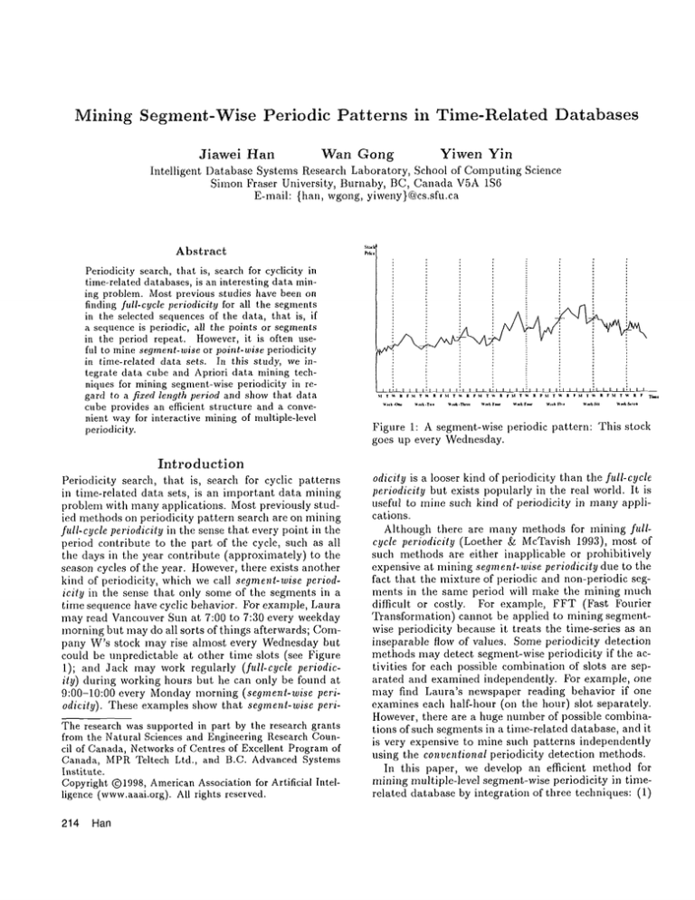
Figure 1: A segment-wise periodic pattern:
goes up every Wednesday.
This stock
Introduction
Periodicity search, that is, search for cyclic patterns
in time-related data sets, is an important data mining
problem with many applications. Most previously studled methods on periodicity pattern search are on mining
full-cycle periodicity in the sense that every point in the
period contribute to the part of the cycle, such as all
the days in the year contribute (approximately) to the
season cycles of the year. However,there exists another
kind of periodicity, which we call segment-wise periodicily in the sense that only some of the segments in a
time sequence have cyclic behavior. For example, Laura
may read Vancouver Sun at 7:00 to 7:30 every weekday
morning but may do all sorts of things afterwards; Company W’s stock may rise almost every Wednesday but
could be unpredictable at other time slots (see Figure
1); and Jack may work regularly (full-cycle periodicity) during working hours but he can only be found at
9:00-10:00 every Mondaymorning (segment-wise periodicity). These examples show that segment-wise periThe research was supported in part by the research grants
from the Natural Sciences and Engineering Research Council of Canada, Networksof Centres of Excellent Programof
Canada, MPRTeltech Ltd., and B.C. Advanced Systems
Institute.
Copyright @1998,AmericanAssociation for Artificial Intelligence (www.aaai.org).All rights reserved.
214 Han
odicity is a looser kind of periodicity than tim fulbcycle
periodicity but exists popularly in the real world. It is
useful to mine such kind of periodicity in many applications.
Although there are many methods for mining fldlcycle periodicity (Loether & McTavish 1993), most
such methods are either inapplicable or prohibitively
expensive at mining segment-wise periodicity due to the
fact that the mixture of periodic and non-periodic segments in the same period will make the mining much
difficult or costly. For example, FFT (Fast Fourier
Transformation) cannot be applied to mining segmentwise periodicity because it treats the time-series as an
inseparable flow of values. Someperiodicity detection
methods may detect, segment-wise periodicity if the activities for each possible combination of slots are separated and examined independently. For example, one
may find Laura’s newspaper reading behavior if one
examines each half-hour (on the hour) slot separately.
However, there are a huge number of possible combinations of such segmentsin a time-related database, and it
is very expensive to mine such patterns independently
using the conventional periodicity detection methods.
In this paper, we develop an efficient method for
mining multiple-level segment-wise periodicity in timerelated database by integration of three teclmiques: (1)
data cube structure (Chaudhuri & Dayal 1997), (2)
bit-mapping technique, and (3) the Apriori mining technique (Agrawal & Srikant 1994). It shows that data
cube structure provides an efficient and effective structure not only for on-line analytical processing (OLAP)
but also for on-line analytical mining.
Notice although the problem of mining segment-wise
periodicity shares some similarity with that of mining
cyclic association rules (Ozden, Ramaswamy,& Silberschatz 1998), our study is not confined to perfect cyclicity but Mlowsperiodicity with certain confidence. Furthermore, the introduction of data cubes and bit-map
techniques improves the efficiency of periodicity mining.
The remaining of the paper is organized as follows.
In Section 2, concepts related to segment-wise periodicity are introduced. In Section 3, methods for mining
segment-wise periodicity in regard to a given length period are studied. In Section 4, we discuss the extension
of the methods. Weconclude our study in Section 5.
Segment-wise periodicity:
concepts
Basic
Given a time series, we denote the ith time as ti, i > 0,
which can be referenced as i. t, where t is the time unit
referring to the time granularity. Weuse 7~ to denote
the ith time unit. That is, T/ is mapped to the time
interval [ti,ti+l),
where i > 0. For any time series,
the ith and the jth time units are called similar with
respect to a time-related attribute if the time-related
attribute values at these two time units fall into the
same category according to a given concept hierarchy.
A cycle is formed if, throughout the whole time series
being examined, there exist (with certain high probability) equally-spaced similar measures of some timerelated attribute. A periodic pattern is the union of a
set of cycles with equal periodic interval. Formally, we
have,
Definition 1 For any given time series whose size is
n, if 3p, o E Z+ (i.e., positive integer), 0 <_ p <
and 0 < o < p and ifVs E Z+,0 < s < nip, the
(p ¯ s + o)th time units are all similar with respect
the time series, we call this a cycle, denoted by C =
(p, o, V), where p is the length or period of the cycle,
o the offset indicating the first time at which the cycle
occurs, and V the concept category of the values that
form the cycle.
[]
Whenthe length of the cycle is known, the cycle can
be denoted in a shorter term as C = (o, V).
Example1 Suppose we have a time series whose sequence,
after mappingthe values into their correspondingcategories,
is 132113412341.Since starting at offset 1, every fourth
position in the sequencerepeats the value 3, there is a cycle
which can be denoted as (4, 1, 3) or *3**. Similarly,
have cycles (4, 3, 1) and (6, 2, 2).
rn
Definition 2 For any given time series whose size is
n, if for some p, m E Z+, 0 < p < n and m > O, 3
m cycles Ci of periodp, 0 <_ i < m, then what these
m cycles formed is a periodic pattern with period p.
The pattern is denoted by P = (p,m,C), where C
{(Oi, Vi)lCi = (p, oi, P~) V 0 <_ i < m}. If the number
cycles in a pattern equals to the pattern length, we refer
to such a pattern as a complete periodic pattern
which can be represented by the pattern sequence itself.
The general type of periodic pattern is consequently referred to as partial periodic pattern.
1:3
Exanaple 2 The sequence given in the previous example
has pattern sequences "3"1 and *’2"**, where pattern "3"1
is the union of cycles (4, 1, 3) and (4, 3, 1). The
terns "3"1 and **2***in the previous examplecan thus be
denotedby (4, 2, {(1, 3), (3, 1)}) and (6, 1, {(2, 2)})
tively. Since not every time unit in these patterns has a
cycle, they are partial periodic patterns. If, presumably,
we found a pattern (3, 3, {(0, 1), (1, 2), (2, 3)}),
corresponding sequence string is 123, we wouldcall such a
pattern a complete pattern,
o
Notice that the periodicity defined above refers to
perfect periodicity in a time series in the sense that all
of the corresponding time units in the series are similar.
This is the ideal case. In practice, most people tolerate
misses. For example, when we say that Jack reads New
York Times every day, we often mean that he does it
almost every day. Therefore, the concept of confidence
of periodicity should be introduced.
Definition
3 A time series contains a cycle C =
(p, o, V) with confidence 7 if the re are 7 × S ti me
units with the period p and the offset o which have the
value V, where S is the numberof periods in the series.
[3
Notice that a perfect cycle in a time series as defined
by Definition 1 implies 7 = 1. Similarly, we can define
confidence for full and partial periodic pattern. Usually, a user or an expert may provide a minimumconfidence threshold, min_conf, to indicate the minimum
strength of the periodicity to be mined. The mining of
segment-wise periodicity is to find all partial and complete periodic patterns satisfying the specified minimum
confidence threshold in a time-series database.
Data cube-based mining of fixed-length
segment-wise periodicity
In this section, we discuss howto construct data cubes
with a given period length (e.g., per year, per day) from
a time-series database and how to use such cubes for
mining segment-wise periodicity.
Data cube construction:
Reference
cube
and working
cube
Example 3 A sales database contains the sales information of a company from January 1993 to December1993,
and there are four attributes: location, product, profit and
time. The first two, location and product, are non-timerelated, profit is time-related, and the time granularity is
month. Supposewe wouldlike to search for quarterly periodicity with respect to the profit in 1993. The confidence
threshold is set as 0.75. The concept hierarchies for time,
KDD-98 215
location, and product are respectively: month ~ quarter
--+ year, city --~ country --~ region, and product-name
--+ product-type. Moreover,profits can be generalized into
several intervals based on an automatically generated numerical hierarchy (Han&Kamber1998).
vI
To facilitate
periodicity mining, we construct two
data cubes, reference cube and working cube, as follows.
First, a set of objects are collected based on the mining query. Associated with each object is a time series of
a time-related attribute (e.g., profit). A reference cube
is built with the time-related attribute (e.g., profit) as
its measure, and with time and tile remaining attributes
as its dimensions. In most cases, the reference cube is
a minimally generalized cube: the concepts of the time
dimension are at a user-preferred finest time granularity; similarly for other dimensions in the reference cube.
Figure 2 shows an instance of a reference cube referring
to the sales database.
"w"
~ :/ e
measurement
(profit)
///
//
Q_
Chicagob6~
Singapore46
..1...
~g
637 804
759
545 837 1319
1047
N.Y. 118: 746
118911~51152
Pori~ 752
799 471 1294
Jan-93 Ftb.93 ....
’ ’ 0~-93 Nov-93 D¢¢.93
Time
Figure 2: A reference cube of Example 3
Tile reference cube provides an efficient structure to
access and index the minimally generalized data. Moreover, each single-dimensional slice of tile cube along the
time dimension represents one time series. For example, the shadedslice shownin Figure 2 is the time series
with respect to (Chicago, Oarry_Bags}. This structure
facilitates the retrieval of time series. With one scan
through tile original relation, each tuple in the taskrelevant data set can be mappedto exactly one cell in
the reference cube, and all the task-relevant data are
transferred into the cube.
Secondly, from tile reference cube we construct a
working cube which includes the dimensions of all nontime-related attributes in the reference cube (location,
product), folds the time-related measure(profit) into an
interval-based (profit) dimension, and folds the time dimension into two: time-index dimension and periodindez dimension. All the dinaension values are generalized to their desired levels according to their corresponding concept hierarchies. The levels chosen are
based on the granularity at which the user would like
to discover and view the periodic patterns. A 3-D slice
of the working cube generated from the reference cube
in Figure 2 is shown in Figure 3, where the location
216 Han
location
product
= Chicago
= carry-
//
/
//
,, / /i//.
4000-5000
(5)
3O00-4000 (4)
2(R30-3OOO (3)
period-Index
1 (R]O-20O0 (2)
O- IOOO(1)
- 1000-0 (0)
1
mo
tittle-index
///
"I
and product dimensions take the value pair (Chicago,
Carry_Bags}.Notice since each cell needs only a bit (existent, nonexistent), each slice of the working cube can
be implementedas a bit-array, except the last slice, period_index = all, which contains tile numberof nonzero
bits of all the other period-index slices and each cell is
an integer.
1
too2
(period
1
2
too3
= quarter)
Figure 3: A T-slice of the working cube generated from
the reference cube.
As shownin Figure 3, the time dimension in the reference cube is reshaped in the working cube into two
dilnensions: One, time-index, refers to the offset in a
given period such as quarter, and the other, periodindex, serves as a dimension for indexing tile periods.
Thus the working cube includes five dimensions: (1) location, (2) prodvct, (3) profit, (4) time-index, and (5)
period index.
In general, a working cube consists of the following
dimensions: time-index, period-index, time-related attribute, and one or more non-lime-related attributes. A
T-slice is a slice of the working cube which includes
the complete time plane and the entire domain of the
time-related attribute dimension. It represents the time
series information of one object and can be encoded by
a bit-array. Our segment-wise periodicity mining will
be focused on the examination of the working cube and
its T-slices.
Mining segment-wise
periodic
patterns
Tile nfining of segment-wise periodic patterns proceeds
as follows. First, the one-cycle periodic patterns is
mined based on the occurrence frequency of a pattern
in tile working cube: a pattern V is a one-cycle pattern
at time_index ti if its occurrenceprobability at ti is not
smaller than the minimum confidence threshold. Second, for k > 1, the (k + 1)-cycle periodic patterns are
mined by growing the k-cycle periodic patterns based
on a method similar to the Apriori principle developed
at miningassociation rules, i.e., a (k+ 1)-cycle is a candidate pattern if all of its k-cycle subsets are k-cycle
patterns. All the (k + 1)-cycle candidates can be verified by scanning the working cube once.
The mining process is illustrated as below.
Algorithm 1 (Mining Periodicity
Patterns)
Find the
complete set of periodic patterns with period p (given) and
confidence threshold 7 in a time series database.
Input: (1) non-time-related attributes
A1, ..., A,; (2)
time-related attribute AT; (3) time attribute, T, bounded
by a time interval; (4) time granularity, g, and a given
period, p, where glP (P is a multiple of g); (5) a time
erarchy and concept hierarchies associated with all taskrelevant attributes; and (6) confidence threshold,
Output: The set of periodic patterns with a period p in
the time series.
Method:¯ Step i: Construction of a reference cube: Constructthe reference cube, based on task-relevant data.
The cube has a time dimension, T, the relevant nontime-related attributes,
A1, ..., A,,, and the timerelated attribute, AT as the measure. Notice that necessary generalization may have been performed for generating the reference cube using the available concept
hierarchies.
¯ Step 2: Construction of the working cube: Transform
the reference cube into a working cube, which preserves
non-time-related dimensions A1, ¯ .., An, converts the
time-related attribute, AT, into an interval-based dimension, and converts the time dimension T, into a
time_index dimension and a period_index dimension,
based on the period p. Each cube cell is boolean except that each cell on the aggregation plane (where
period_index = all) is an integer, count.
¯ Step 3: Mining periodic patterns: For each time series,
represented by a T-slice, do the following.
.pl = FindOneCyclePatternsO;
FOR(i=2;i<p&Pi-1
~i~;i++)
C79i := FormCandidatePatternSet(i);
pi := CheckPatternExistenee(C79i);
}
/* END FOR */
RETURN
Periodic pattern
set 79 := Ui=x
p 79i.
ca
The three functions in Step 3 are explained below.
FindOneCyclePatterns
finds frequent 1-cycles in the
working cube W[Time, Period, Value]. A one-cycle periodic pattern is detected if there is a cycle C = (p, o, V)
with a confidence no less than min_conf, where p is the
cycle length (i.e. period), o the offset, and V the value.
In a T-slice of the working cube, the time_index corresponds to the offset o, the size of the lime_index corresponds to the period p, and the size of period index
is the total number of periods occurring in the time
series. An event is frequent if it occurs no less frequent than rnin_conf x Iperiod_indexl.
This process
is performed by scanning once only the slice where period_index - all and checking whether the count is no
less than min_con f × Iperiod_indexl.
Example 4 The one-cycle patterns
of Example 3 can be
computed by searching through the slice period_index = all
of the T-slice of the working cube (Figure 4). Since the
number of periods (quarters) = 4, and rain_coal= 0.75, any
summary cell with a count no less than 4 x 75% = 3 will
pass the test. Three cells: (month --- 1, profit = 1), (month
= 2, profit = 1), and (month= 3, profit ---- 2), pass the cycle
test. That is, Co = (3, 0, 1), C1 = (3, 1, 1), and C~ =
location = Chicago
product= carry-bag
period-index
= all
profit
4OOO-5OOO
(5)
3000-4000(4)
2009-3000(3)
1000-2000
(2)
0-1000(1)
3
-1000-0(0)
1
1
3
4
mol too2 mo3
time-index(period= quarter)
Figure 4: A slice
where "period_index
= alp
2, 2). The output from the algorithm is thus 79~ = {Po~ =
(3, 1, {(0, 1)}), 2 = (3, 1, {(1, 1)} ), P0a= (3, 1, {(2, 2)})}
FormCandidatePat
ternSet
finds frequent /-cycle candidates in the working cube
W[Time, Period, Value] from a set of frequent (i - 1)cycles.
We observe an interesting
property for cycle growth
which is similar to the Apriori property at mining association rules (Agrawal & Srikant 1994): if a k-cycle
is frequent (i.e.,
passing the min_conf threshold), all
its j-itemset for j < k must be frequent as well. This
leads to the following algorithm which forms the candidate/-cycle
patterns,
denoted by C~oi, from a set of
(i- 1)-cycle patterns (7)i-1).
The procedure contains
two phases: a join phase and a prune phase. The join
is done on the (i - 1)-cycle pattern set )/-1 t o f orm a
candidate/-cycle
pattern set C7)i. The prune phase discards those candidate patterns in C7) i that have some
(i- 1)-cycle subpatterns which are not in 7)i-1. This
is shown in the example below.
Example 5 We continue working on the 1-cycle periodic patterns,
791, obtained in Example 4. The join
of 791 and 79a yields 2-cycle candidate patterns CP~ =
(3, 2, {(0,1),(1,1)}),
CP? = (3, 2,{(0,1),(2,2)}),
CP~ = (3,2, {(1, 1), (2, 2)}). (Note: none of these
dates will be pruned since all of their 1-cycle subpatterns
are actual patterns). Suppose the 2-cycle periodic patterns
found after verification
are Pg=CP~I and P~=CP~. The
only candidate 3-cycle periodic pattern formed from P~ and
P~ is then CP0a=(3, 3, {(0,1),(1,1),(2,2)}).
This candidate
is eliminated by pruning because a subpattern of C’P0a, (3, 2,
{(0,1), (1,1)}), does not belong to the set of 2-cycle patterns.
[3
CheckPatternExistence
checks the working cube to
verify whether the pattern posted in the/-cycle
candidate set is frequent.
After deriving the /-cycle
candidate patterns,
we
check whether such candidates form real /-cycle patterns in the working cube. This is done by checking
whether the number of simultaneous occurrences of the
/-cycles in a candidate pattern in a T-slice exceeds the
minimum confidence threshold.
When a pattern is confirmed, all of its subpatterns are eliminated from the
pattern lists of fewer cycles.
KDD-98 217
Since the candidate pattern list can be encoded as a
bit plane in the time-series slice of the working cube,
the verification process can be implementedefficiently:
For each period-index slice, a bit-and of the two planes
will verify which candidate pairs are valid on a particular period-index plane. It takes only ]period_index]
bit-and operations plus the pair-counting and threshold
checking to accomplish it.
Our performance study (not included here for lack
of space) shows that our method is more efficient than
either (1) using Apriori only without exploring the bitarray cube structure or (2) using tile cube structure but
not exploring the Apriori principle.
Discussion
Mining multiple-level
cyclic
patterns
With the reference cube structure, the method can be
easily extended to mining cyclic patterns at multiple
levels of abstraction.
For the non-time-related dimensions, such as location
and product, a multi-level reference cube can be built by
incorporation of multiple levels of granularities in cube
construction. Such a reference cube consists of a group
of cuboids, each representing a combination of particular levels of location and product. One maymine cyclic
patterns for each combination of city and product and
then roll-up to find patterns for each country and product category. The same is true for the time dimension.
One may drill along the time hierarchy to mine cyclic
patterns from quarterly to monthly, weekly, or yearly.
This notion of multi-level mining can be extended to
time-related measure, such as profit, in the reference
cube. Drilling can be performed on the time-related
measures to mine periodicity at multiple granularities.
Notice that for time-related measures, there is an interesting relationship amongdifferent levels of granularity under the same confidence threshold: if a pattern
is cyclic with a certain period p, the pattern must be
cyclic with the same period p at a rougher scale. For
example, if the sales profit for shoes in Paris in 1993
counted in the unit of thousands forms a cyclic patterns by quarter, then tile same profit, when counted
in tens of thousands, still forms a cyclic pattern. This
property can be used to first explore tile periodicity at
a rough scale, and then progressively drill-down on tile
discovered periodic patterns to see whether they are still
periodic at a refined scale. Drilling can be performed
efficiently with tile data cube structure.
Mining cyclic patterns with arbitrary
length of periods
Mining cyclic patterns under a given period covers a
large number of applications since people often like
to mine periodic patterns for natural periods, such as
annually, quarterly, monthly, weekly, daily, or hourly.
However, the periodicity may appear at some unexpected periods, such as every 11 years, or every 13
218 Han
hours. It is interesting to provide facilities to mineperiodicity for all the possible periods.
One simple extension to our technique for mining
segment-wise periodicity for arbitrary length of periods
is to repeatedly apply our algorithm for a growing sequence of periods. That is, one may put the algorithm
in a for-loop and set the for-loop index as the period p
from 1 up to the entire length of the time series. This
technique, though straightforward, mayrequire a lot of
processing power.
If the confidence threshold is 1 (perfect periodicity),
many properties
explored in (Ozden, Ramaswamy,
Silberschatz 1998) can be adopted to reduce the search
effort. For example, if a time series is periodic with a
period of p, it is periodic for any multiples of p. This implies that one maysearch for segment-wise periodicity
from small periods up, cross-out all the multiples of a
period along the way to reduce the search effort. Unfortunately, such nice properties do not exist for imperfect
cycles. More sophisticated techniques are needed to be
developed to reduce the search space.
Conclusions
Segment-wiseperiodicity, which counts the cyclicity behavior of every possible time segment in a time-related
database, represents a more general notion than the full
periodicity studied popularly on time-related data.
In this paper, we developed a efficient method for
mining segment-wise periodicity with a fixed length period, which exploring data cube, bit-arrray, and the
Apriori mining techniques. The method constructs
working cubes from a time-series reference cube based
on the given period and the dimensions to be analyzed.
The working cube can be implemented using a bit-array
technique and the mining adopts an Apriori-like, levelwise mining technique. Our study shows that data cube
provides an efficient structure and a convenient way for
interactive mining of multiple-level periodicity.
It is important to extend the method for mining
segment-wise periodicity for arbitrary length period. A
study of this extension will be reported in a coming
paper.
References
Agrawal, R., and Srikant, R. 1994. Fast algorithms for
mining association rules. In Proc. 1994 Int. Conf. Very
Large Data Bases, 487-499.
Chaudhuri, S., and Dayal, U. 1997. An overview of
data warehousing and OLAPtechnology. ACMSIGMOD
Record26:65-74.
Hun, J., and Kamber, M. 1998. Data Mining: Concepts
and Techniques. in preparation.
Loether, H. J., and McTavish,D. G. 1993. Descriptive and
Inferential Statistics: An Introduction. Allyn and Bacon.
Ozden, B.; Ramaswamy,
S.; and Silberschatz, A. 1998.
Cyclic association rules. In Proc. of 1998Int. Conf. Data
Engineering (ICDE’98), 412-421.