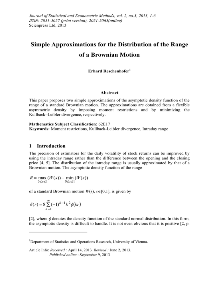
Journal of Statistical and Econometric Methods, vol. 2, no.3, 2013, 1-6
ISSN: 2051-5057 (print version), 2051-5065(online)
Scienpress Ltd, 2013
Simple Approximations for the Distribution of the Range
of a Brownian Motion
Erhard Reschenhofer1
Abstract
This paper proposes two simple approximations of the asymptotic density function of the
range of a standard Brownian motion. The approximations are obtained from a flexible
asymmetric density by imposing moment restrictions and by minimizing the
Kullback–Leibler divergence, respectively.
Mathematics Subject Classification: 62E17
Keywords: Moment restrictions, Kullback-Leibler divergence, Intraday range
1 Introduction
The precision of estimators for the daily volatility of stock returns can be improved by
using the intraday range rather than the difference between the opening and the closing
price [4, 5]. The distribution of the intraday range is usually approximated by that of a
Brownian motion. The asymptotic density function of the range
R  max (W ( s ))  min (W ( s ))
0  s 1
0  s 1
of a standard Brownian motion W(s), s[0,1], is given by

 ( r )  8  ( 1) k 1 k 2 kr 
k 1
[2], where  denotes the density function of the standard normal distribution. In this form,
the asymptotic density is difficult to handle. It is not even obvious that it is positive [2, p.
1
Department of Statistics and Operations Research, University of Vienna.
Article Info: Received : April 14, 2013. Revised : June 2, 2013.
Published online : September 9, 2013
2
Erhard Reschenhofer
430]. Moreover, its numerical instability for small values of r is also a serious issue. Thus,
only simple measures such as E(R2) are used in quantitative finance. To enable more
complex applications, the next section proposes two approximations of (r) which are
both easier to handle and numerically stable. Section 3 concludes.
2 Approximations
The density  is approximated by densities of the form
h( x )  I ( ,  ] ( x )
p
e
(
x p
)

( 1p )


 I (  , ) ( x )
h1 ( x )
(1   ) q  ( x   )q
,
e
( 1q )


h2 ( x )
where   1.34577 is the mode of  and p,q,,>0, 0<<1 are unknown parameters.
Using for m>0

m xp
x e
dx 
( mp1 )
p
0
[3, p. 337], we obtain
E( X ) 

( 1p )

 xe
0
(
 (    z) e
( 1p ) 
 ( 2p )
E X 


p
  

p
( 1p )
m

p
0
( 1p )

x p
)

dx 
zp
 (1   )
p

( 1p )

(  ) dz 
( 1p )
,
( 1q )
m
 (   x) e
p

(1   ) q 
 zq
(



z
)
e
 dz

( 1q ) 0
 ( q2 )
m z
 ( z ) e (  ) dz 
 ( mp1 ) m
(1   ) q   ( x   )q
dx
 xe
( 1q ) 
(
x q
(1   ) q 
m (  )
(
x


)
e
dx

( 1q ) 
(1   ) q 
m  zq
(
z

)
e  dz

( 1q ) 0
(1   ) ( mq1 ) m
( 1q )
x p
)

dx 
,
and
Var( X )  E ( X   ) 2  ( E ( X )   ) 2
Simple Approximations for the Distribution of the Range of a Brownian Motion

 ( 3p ) 2
( 1p )
(1   ) ( q3 ) 2

( 1q )
3
2

 ( 2p )
 ( q2 ) 
 .

 
 (1   )

( 1p )
( 1q ) 


The continuity restriction
h1 (  ) 
p
( 1p )

(1   ) q
 h2 (  )
( 1q )
implies that

(1   ) q( 1p )
 p( 1q )

and the unbiasedness restriction
 ( 2p )
E( X )    
( 1p )
 (1   )
 ( q2 )
( 1q )
2
2

 E ( R)
that

  2


2

 ( 2p ) 
( 1q )

.
 
( 1p )  (1   ) ( q2 )

Thus,


  )  (1   ) q( 1p )
 ( 1q ) ( 2p ) 



(1   ) ( q2 )   p ( 1q )
(1   ) ( 1p ) ( q2 ) 


( 1q ) (2
2
1

 p ( 1p )  2 ( 1q ) (2
2

 )
(1   ) 2 q  2 ( 1p ) ( q2 )  2 p  2 ( 1q ) ( 2p )
.
Noting that
E ( R)  2
E ( R 2 )  4 log(2) , E ( R 3 ) 
2
 ,
2
3
2 3 , E ( R 4 )  9  (3)
[5], where

 (3)   j  3  1.2020569
j 1
(for tables of values of the Riemann zeta function  see [1]), and imposing in addition the
higher order restrictions
E( X   ) 
2
E( X 3 ) 
 ( 3p ) 2
p
( 1p )


(1   ) ( q3 ) 2
( 1q )
p
 4 log(2)  4
(1   ) q 
  2  E ( R   )2 ,
2

q
(    z ) 3 e  z dz 
(    z ) 3 e  z dz


1
1
( p ) 0
( q ) 0
4
Erhard Reschenhofer
 3 

( 1p )
 3  (
2
2 )  3 2 ( 3 )   3 ( 4 )
p
p
p


(1   )
3 2 ( q2 )  3 2 ( q3 )   3 ( q4 )
1
( q )

2
3


2 3  E ( R 3 ) ,
and
E( X   ) 
4
 ( 5p ) 4
( 1p )

(1   ) ( q5 ) 4
( 1q )
 9 (3)  83 2 3   24 log(2)  2  8
2

3  4
 E(R   )4
yields:
=0.4045,  =0.7544, =0.3466, p=2.879, q=1.525.
(1)
Alternatively, all unknown parameters (except  which is determined by the continuity
restriction) can be selected by minimizing the Kullback-Leibler divergence
DKL ( h)    ( x )
 ( x)
h( x )
dx
of h from . Using [0.385,7] as the interval of integration, we obtain
=0.4090, =0.7600, =0.3478, p=2.920, q=1.539.
(2)
Figure 1 shows that both (1) and (2) approximate  very well. Minor discrepancies occur
only when  is practically zero.
3 Conclusion
The approximations of the asymptotic distribution of the range of a standard Brownian
motion W(s), s[0,1], which have been obtained in the previous section, are probably
good enough for all practical purposes. However, whether they are also simple enough
must be determined in each individual case. A major challenge for future research is to
find an application where only the approximations allow the derivation of an analytic,
closed-form solution of a relevant problem.
5
0.6
0.8
1.0
Simple Approximations for the Distribution of the Range of a Brownian Motion
0.0
0.2
0.4
(a)
2
3
4
5
6
7
1e-04
1
1e-10
(b)
1
2
3
4
5
6
7
Figure 1: Normal approximation (blue) and new approximations (1: yellow, 2: green) of
the asymptotic density function (red) of the range of a standard Brownian motion on [0,1].
(a): Linear scale, (b): Log scale
6
Erhard Reschenhofer
References
[1]
[2]
[3]
[4]
[5]
M. Abramowitz and I.A. Stegun, Handbook of mathematical functions with formulas,
graphs, and mathematical tables, National Bureau of Standards, 1964.
W. Feller, The asymptotic distribution of the range of sums of independent random
variables, The Annals of Mathematical Statistics, 22, (1951), 427-432.
A. Jeffrey and D. Zwillinger (eds.), Gradshteyn and Ryzhik's table of integrals,
series, and products, Seventh edition, Academic Press, 2007.
M.B. Garman and M.J. Klass, On the estimation of security price volatilities from
historical data, The Journal of Business, 53, (1980), 67-78.
M. Parkinson, The extreme value method for estimating the variance of the rate of
return. The Journal of Business, 53, (1980), 61-65.