Exploring Similarities in Music Performances with an Evolutionary Algorithm
Søren Tjagvad Madsen and Gerhard Widmer
Austrian Research Institute for Artificial Intelligence
Vienna, Austria
Department of Computational Perception
University of Linz, Austria
Abstract
The paper presents a novel approach to exploring similarities in music performances. Based on simple measurements
of timing and intensity in 12 recordings of a Schubert piano
piece, short ‘performance archetypes’ are calculated using a
SOM algorithm and labelled with letters. Approximate string
matching done by an evolutionary algorithm is applied to find
similarities in the performances represented by these letters.
We present a way of measuring each pianist’s habit of playing
similar phrases in similar ways and propose a ranking of the
performers based on that. Finally, an experiment revealing
common expression patterns is briefly described.
Introduction
Expressive music performance as the artistic act of ‘shaping’
a given piece of written music has become a topic of central interest in the fields of musicology and music psychology (Gabrielsson 1999). In classical music, in particular,
the performing artist is an indispensable part of the system,
shaping the music in creative ways by continually varying
parameters like tempo, timing, dynamics (loudness), or articulation, in order to express his/her personal understanding
of the music. Musicologists and psychologists alike would
like to understand the principles of this behaviour – how
much of it is determined by the music, whether there are
unwritten rules governing expressive performance, etc. Recently, also AI researchers have started to look into this phenomenon and to apply their techniques (e.g., machine learning) to get new insights into patterns and regularities in expressive performances (López de Mántaras & Arcos 2002;
Widmer et al. 2003).
In this paper, we present an evolutionary algorithm for
finding approximately matching substrings in character sequences, and use it to search for structure in expressive performances (by famous pianists) encoded as strings. The goal
is to study both the artists’ intra-piece consistency and potential similarities between their playing styles.
It is known (and has been shown in laboratory experiments) that performing expressively in a stable manner is
a way of emphasising the structure of the music (Clarke
1999). In particular, similarities in timing patterns across
c 2005, American Association for Artificial IntelliCopyright gence (www.aaai.org). All rights reserved.
Index
Pianist
Recording
Year
0
1
2
3
4
5
6
7
8
9
10
11
Barenboim
Brendel
Gulda
Horowitz
Kempff
Leonskaja
Lipatti
Maisenberg
Pires
Rubinstein
Uchida
Zimerman
DGG 415 849-2
Philips Classics, 456 061 2
Paradise Productions 9/99
Columbia MS 6411
DGG 459 412-2
Teldec 4509-98438-2
Emi Classics CDH 5 65166 2
Wiener Konzerthaus KHG/01/01
DGG 457 551-2
BMG 09026 63054-2
Philips 456 245-2
DGG 423 612-2
1977
1972
1999
1962
1965
1995/96
1950
1995
1996
1991
1996
1990
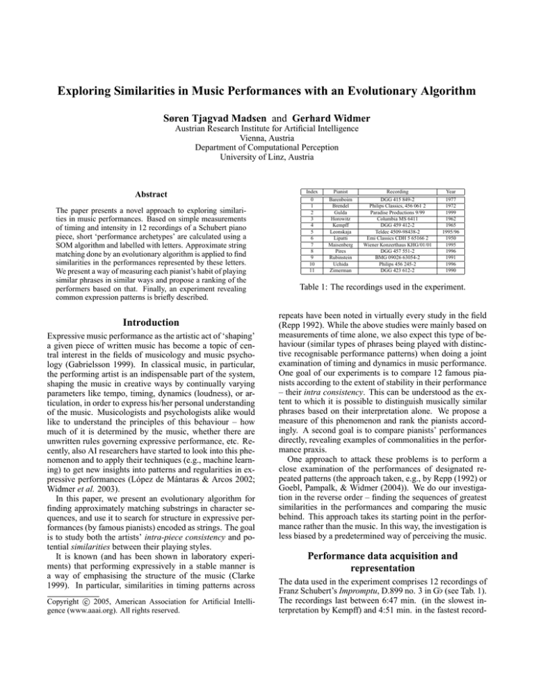
Table 1: The recordings used in the experiment.
repeats have been noted in virtually every study in the field
(Repp 1992). While the above studies were mainly based on
measurements of time alone, we also expect this type of behaviour (similar types of phrases being played with distinctive recognisable performance patterns) when doing a joint
examination of timing and dynamics in music performance.
One goal of our experiments is to compare 12 famous pianists according to the extent of stability in their performance
– their intra consistency. This can be understood as the extent to which it is possible to distinguish musically similar
phrases based on their interpretation alone. We propose a
measure of this phenomenon and rank the pianists accordingly. A second goal is to compare pianists’ performances
directly, revealing examples of commonalities in the performance praxis.
One approach to attack these problems is to perform a
close examination of the performances of designated repeated patterns (the approach taken, e.g., by Repp (1992) or
Goebl, Pampalk, & Widmer (2004)). We do our investigation in the reverse order – finding the sequences of greatest
similarities in the performances and comparing the music
behind. This approach takes its starting point in the performance rather than the music. In this way, the investigation is
less biased by a predetermined way of perceiving the music.
Performance data acquisition and
representation
The data used in the experiment comprises 12 recordings of
Franz Schubert’s Impromptu, D.899 no. 3 in G[ (see Tab. 1).
The recordings last between 6:47 min. (in the slowest interpretation by Kempff) and 4:51 min. in the fastest record-
GJNDVJRIKRLJPJVDBCUCCPVNTJCPNJLJQCPCCSUT
JJQSNJGXBCNVMICFMRNFXVMOJPMTGNBUQTHUGECB
CUIRIJCBCUIRORNSGSQVNHLIHHUYFXKDQJROBTQJ
PJVJIDQCCRUTNJVNRDCPQJCPRTGHHJCPVOHHQJBV
QGTSRTGRGW
A
B
C
D
E
F
G
H
I
J
K
L
M
N
O
Figure 2: Elisabeth Leonskaja playing the Impromptu.
P
Q
R
S
T
U
V
W
X
Y
resented by 2 letters (which is appropriate, given the rather
sparse melodic content of the music). A performance of the
complete impromptu then looks like the 170 letters shown
in Fig. 2.
Finding similarities in the performances can now be expressed as a string matching problem or an approximate
string matching problem, which is the main subject of this
paper.1 The approximate string matching is done with an
evolutionary algorithm described below. We will refer to
the task of finding all similar non-overlapping strings in a
performance (up to a similarity threshold) as segmenting the
string, yielding a segmentation of the performance.
Figure 1: The performance letters: atomic motions in the
tempo-loudness space (end points marked with dots).
ing by Lipatti. The 12 recordings were semi-automatically
‘beat-tracked’ with the aid of appropriate software (Dixon
2001). The onset time of each beat was registered and for
each beat a local tempo in beats per minute was computed.
Furthermore the dynamic level at each beat tracked was also
computed from the audio signal.
For each beat in the score, we now have measurements
of tempo and loudness, forming a bivariate time series.
The performances can be described as consecutive points
in the two dimensional tempo-loudness space as suggested
by Langner & Goebl (2003). This discretised version of
the data captures the fundamental motions in the tempoloudness space and thereby hopefully the fundamental content of the performances. Accentuations between the points
of measurements are however not present in the data. Neither are refinements of the expression such as articulation
and pedalling.
Performance letters
To explore patterns in the performances, we want to discover
similar sequences in the points measured. A way to achieve
this is through the notion of performance letters (Widmer
et al. 2003). A performance letter describes one ‘generic’
motion in the tempo-loudness space, in this case between
three points. To derive these, the series of points from each
of the 12 performances were divided into sections of three
points each, the end point of a sequence being the beginning
of the next. All the short sequences were then clustered into
a 5×5 grid according to similarities using a self organising
map (SOM) algorithm, resulting in 25 ‘archetypes’ representing the most prominent performance units in the corpus. The process is described in (Widmer et al. 2003). The
archetypes were labelled with letters – the performance letters (Fig. 1). A distance matrix quantifying the differences
between letters was output as well.
The performances can now be approximately represented
as a string of performance letters. Since the beats were
tracked at the half note level (the piece is notated in 4/2
time) and a letter spans three beats, one bar of music is rep-
Measuring consistency
As a tool for measuring the consistency, a structural analysis of the piece was performed (by the authors), dividing the
piece into similar subsections (phrases) based on the musical content alone. The Impromptu can be seen to consist of
15 phrases of varying length (1 to 4 1/2 measures) and up
to 6 occurrences. The analysis serves as a lookup-table for
asking if two performance substrings are applied to similar
musical content: this is the case if they cover corresponding
sections of two occurrences of the same phrase type.
Measuring consistency is done in two steps: finding a
string segmentation based on performance similarities and
evaluating how well the segmentation corresponds to similar
music. A performer distinguishing every type of phrase with
individual expressions will result in a ‘perfect’ segmentation
and therefore a perfect evaluation. More precisely, given a
segmentation of a performance, all similar strings are examined to see if they are applied to similar music. The ‘correct’
corresponding letters are counted as true positives (TP). The
current analysis allows a maximum of 163 of the 170 letters to be matched to similar musical content. If a string is
found to not correspond musically to another string to which
it is considered similar, the letters in the string are counted
as false positives (FP).
Given different segmentations, we can now measure how
well they correspond to the structure of the music. We express this in terms of recall and precision values (van Rijsbergen 1979). Recall is the number of correctly found letters
(TP) divided by the total number of letters there is to find in
an ‘optimal’ segmentation (in this case 163). Precision is TP
divided by the total number of matching letters found (TP +
FP). The F-measure combines recall and precision into one
value (an α of 0.5 used throughout this paper giving equal
1
It has recently been shown that a machine can also learn to
identify artists on the basis of such strings (Saunders et al. 2004).
90
Pos. 3
Tempo
Loudness
10
70
60
50
40
5
40
60
Tempo
30
80
0
10
5
10
60
Tempo
80
0
5
Beats
10
Figure 3: Two instances of the letter sequence ‘LHPTB’ from Rubinstein’s performance plotted in the tempoloudness space (left) and each dimension separately (right).
weight to precision and recall):
F (R, P ) = 1 −
α P1
From this first attempt it looks as if the pianists are playing rather inconsistently, only occasionally repeating a short
performance pattern. Segmenting the performances based
on exact matching might be expecting too much concistency
of the performer and indeed expecting too much of the discrete approximate representation of the performance. On the
other hand, longer strings do occur so the performance letters seem to be able to represent some characteristics in the
performances. We will now explore the possibilities of finding similar patterns based on inexact string matching.
Evolutionary search for similar strings
10
5
Pos. 111
40
5
Beats
Pos. 3
Pos. 111
15
Loudness
15
Loudness
Pos. 3
Pos. 111
80
15
1
, 0≤α≤1
+ (1 − α) R1
(1)
As precision and recall improve, the F-measure reflecting
the inconsistency drops. It weights the number of correct
corresponding letters found against their ‘correctness’.
String matching
To inspect the performances for distinguishable patterns, we
now are interested in finding recurring substrings in the performances. A natural way to start this task was to apply an
exact string matching algorithm. The S EQUITUR algorithm
(Nevill-Manning & Witten 1997) that identifies hierarchical
structure in sequences was applied to each string.
Distinctive similarities in the performances do not show
right away. The algorithm found mainly very short sequences and many letters were not included in any sequence.
Even though the longest repeated patterns found in all of the
performances spanned 5 letters (2 1/2 measures of music),
some of the performances only contained repeated strings of
2 and 3 letters. Fig. 3 shows 2 occurrences of a 5 letter pattern found, plotted in the tempo-loudness space as well as
tempo and loudness separately. The performances look less
similar in the tempo-loudness space due to the accumulated
inaccuracies from the two dimensions.
The two long sequences do refer to similar phrases in the
music. Most of the strings found similar were however not
referring to the same music. With no exception, the number of true positives was smaller than the number of false
positives (precision below 0.5). The segmentations of the
performances by Lipatti and Rubinstein were found most
precise (45.5 % and 43.5 % respectively). Also the greatest
recall rates were found in these performances, which therefore score the best (lowest) F-measures (0.652 and 0.686).
We developed an evolutionary algorithm as a search algorithm able to find inexact matches. The algorithm maintains
a population of similarity statements. A similarity statement
is essentially a ‘guess’ that two substrings of equal length
found in the input string(s) are similar. The evaluation function decides which ones are the most successful guesses.
The best guesses are selected for the next generation and
by doing crossover and mutation in terms of altering the
guesses (dynamically changing the size and position of the
strings) the algorithm can enhance the fitness of the population. After some generations the algorithm hopefully settles
on the globally fittest pair of strings in the search space.
The fitness function has to optimise the string similarity
as well as prefer longer strings to shorter ones. It performs
a pairwise letter to letter comparison of the letters in the
strings and sums up the distances based on the distance matrix output in the clustering process. This is the actual string
similarity measure. The string size also contributes to the fitness in such a way that longer strings are valued more highly
than shorter ones. This is to bias the algorithm towards considering longer less similar strings to short exact ones. The
fitness is calculated from these factors. The amount of advantage given to longer strings is decided based on experiments described below.
Segmenting a performance now consists in iteratively
finding similar passages in the performance string. In each
iteration we run the EA and obtain a fittest pair of strings
and their fitness value. A manually set threshold value determines if the fitness is good enough to let the strings be
part of the segmentation and claimed similar. If they are, a
search for more occurrences of each of the strings is executed. When no more occurrences can be found, the strings
are substituted in the performance data structure with a number identifying this type of performance pattern (equal to the
iteration in which they were found). Further searches in the
data can include and expand these already found entities.
The evaluation of the different objectives we want to optimise (letter similarity and string length) have to be combined
into one single value, so the adjustment of the parameters
as well as the overall threshold is an important and critical
task. Setting the parameters too conservatively, leaving no
room for near matches, would make the algorithm behave as
an exact matching algorithm. On the other hand, allowing
too much difference would make the algorithm accept anything as similar. Selecting the parameters which result in the
lowest F-measure gives an ‘optimal’ segmentation where the
similar strings found have the highest degree of consistency.
1
Mean F−measure
Mean Recall
Mean Precision
Recall, Precision, F−Measure (α = 0.5)
0.9
0.8
0.7
Iteration
(Length)
Start
pos.
Strings found
similar
1
(18)
2
(8)
3
111
22
38
134
78
86
DVJRIKRLJPJVDBCUCC
DQJROBTQJPJVJIDQCC
VNTJCPNJ
UTJJQSNJ
VNRDCPQJ
CBCUIR
CBCUIR
3
(6)
0.6
Iteration
(Length)
Start
pos.
Strings found
similar
4
(8)
5
(4)
142
150
57
62
66
94
159
164
CPRTGHHJ
CPVOHHQJ
RNFX
MOJP
MTGN
NSGS
VQGT
RTGR
0.5
0.4
Table 2: A segmentation of the performance by Leonskaja.
0.3
0.2
70
0.1
0
0.05
0.1
0.15
0.2
0.25
Average dissimilarity allowed
0.3
0.35
Tempo
60
0
50
Pos. 22
Pos. 38
Pos. 134
40
Figure 4: Finding optimal parameters for segmenting the
performance by Leonskaja. The points plotted represent the
average value over 10 runs with ADA value.
30
0
2
4
6
8
Beats
10
12
14
16
6
8
Beats
10
12
14
16
This is the approach taken here.
It turns out that each performance has different optimal
parameter settings – reflecting the degree of variance in the
performance. One way of comparing the consistency in the
performances would be to find the individually optimal settings for each pianist and then compare the respective Fmeasure values. We chose however for this experiment to
optimise the parameters for a single performance, and use
those to segment the remaining performances. This allows
us to compare the segmentations more directly, since the
same similarity measure is used for all performances.
Experiments
Adjusting the fitness function
We want to select the parameters in the fitness function and
the threshold in such a way that sufficiently similar strings
are accepted and too different ones rejected. We would like
to draw this line where the strings found similar are as consistent as possible, i.e., located where the music is similar.
Using the F-measure as a consistency measure, we can
run the algorithm with different parameter settings and evaluate the segmentation. Since the search algorithm is nondeterministic, it is necessary to run every experiment more
than once in order to be certain that a segmentation was not
just an occurrence of bad or good luck.
We saw above that segmenting according to exact matches
was apt to point out numerous small sequences, and the
consistency problems with that. When searching for near
matches, strings of short length (2-3 letters) are still likely
to be similar to too many passages in the performance and
hence not show what we are searching for. The problem
with short sequences is that many of them are not distinctive
enough to characterise only a single musical idea or phrase,
and therefore can be found in more than one context.
As a consequence, we simply terminate the segmentation
if the best string found is of length 2. However, in addition
we try to encourage the EA to select longer strings, by allowing a certain degree of dissimilarity. This is implemented as
a single parameter – a fitness bonus per letter in the strings
Loudness
25
Pos. 22
Pos. 38
Pos. 134
20
15
10
5
0
2
4
Figure 5: The patterns starting at positions 22 (VNTJCPNJ)
and 38 (UTJJQSNJ) refer to similar music; the music at
pos. 134 (VNRDCPQJ) is somewhat different.
under consideration. The value of this parameter is in effect allowing a certain dissimilarity per letter. The question
is what value this parameter – which we will call average
dissimilarity allowed (ADA) – should be given.
The performance by Leonskaja (who is one of the less
known pianists) was sacrificed for adjusting the fitness function. The normalised letter distance matrix contains values
in the interval [0;1]. Generally there is a distance of 0.17–
0.39 between letters next to each other on the normalised
5×5 SOM. The ADA value was gradually increased from
0.01 to 0.35 in steps of 0.01. Fig. 4 shows for each value
of ADA the average F-measure, precision, and recall value
calculated over 10 segmentations with the EA.
Allowing only little dissimilarity makes the algorithm behave in a conservative way – in a run with ADA = 0.1 only 4
strings were found with a total of 32 letters, but 26 of them
being consistent. When ADA is above 0.3, the segmentation
is dominated by a few, but very long strings covering almost every letter in the string, not discriminating very well
the sections in the music. The best average F-measure was
obtained with ADA = 0.21. A segmentation in this setting
found 5 categories of repeated strings of length 4 to 18 (see
Tab. 2). Even though the strings may seem very different,
the number of true positive matches of the letters in Tab. 2
was 80 and the number of false positives 32, giving a recall
of 0.491, precision of 0.714 and F-measure of 0.418.
The strings from iteration 2 were found in 3 occurrences,
F-measure
St. dev F-m
Pianist
0.725
0.765
0.717
0.803
0.606
0.636
0.539
0.535
0.505
0.340
0.390
0.336
0.368
0.427
0.460
0.478
0.540
0.555
0.567
0.597
0.678
0.761
0.000
0.091
0.049
0.029
0.084
0.042
0.044
0.044
0.093
0.050
0.075
Barenboim
Horowitz
Lipatti
Maisenberg
Kempff
Uchida
Brendel
Rubinstein
Pires
Zimerman
Gulda
30
80
Tempo
Precision
0.613
0.538
0.478
0.408
0.459
0.361
0.380
0.366
0.338
0.308
0.172
25
60
Pos. 0
Pos. 108
0
5
10
15
20
25
30
25
30
Beats
16
15
Pos. 0
Pos. 108
14
10
Table 3: Ranking the pianists according to consistency.
5
plotted in Fig. 5: Two of them refer to similar phrases, and
the last (starting at pos. 134) to another phrase (although
some resemblance can be argued). These three strings thus
contribute 16 TPs and 8 FPs. It looks as if Leonskaja is more
consistent in the loudness domain than in the tempo domain
when playing this repeated phrase. The patterns found in
iterations 1 and 3 are also applied to similar phrases.
70
50
20
Loudness
Recall
1
2
3
4
5
6
7
8
9
10
11
Loudness
Rank
12
10
8
6
0
2
4
Beats
6
8
0
5
10
15
20
Beats
Figure 6: a) Gulda playing a short pattern in 10 different variants (loudness plotted only). The two ‘consistent’
performances are intensified. b) Horowitz playing a long
pattern in 2 very similar ways (tempo and loudness plotted separately): FNLLIJPTGRGIRONOH at pos. 0 and
FNMLGJROGRGHRLGOH at pos. 108.
Ranking the performances
All performances were then segmented 10 times with an
ADA value of 0.21. This should tell us how consistent the
performances play under the same measuring conditions.
A ranking according to the average F-measure is shown in
Tab. 3. This suggests that Barenboim and Horowitz are the
most consistent performers of this piece. A Horowitz performance was segmented with the overall single best F-measure
of 0.309. The segmentation of Maisenberg gave the highest
precision, but a mediocre recall result in a lower ranking.
Gulda stand out by receiving the lowest score. His segmentation often results in three types of strings, one of which
is the largest source of confusion. It consists of 4 letters
and occurs 10 times, where only 2 refer to similar phrases.
Fig. 6a) shows the 10 sequences found similar by the similarity measure, plotted in the loudness space. It looks as
if Gulda is not phrasing the music in long sections. Certainly he does not play distinctively enough for the phrases
to be recognised with this similarity measure. Fig. 6b) on the
other hand shows a beautiful example of consistent music
performance: Horowitz playing the beginning of the piece
compared to when he plays the repeat of the beginning.
When listening to Gulda and Horowitz the authors find
that concerning tempo, Horowitz sounds like having a large
‘momentum’ behind the accellerandos and ritardandos – no
sudden changes. Gulda on the other hand is much more
vivid, taking fast decisions in tempo changes. This might
account for some of the difference in consistency measured.
The ranking is not to be taken too literally – the standard
deviation values shown indicate uncertainties in the ranking.
Other parameter settings lead to some changes in the ranking
as well, but our experiments do reflect a general tendency:
Barenboim, Horowitz, Lipatti, and Maisenberg seem to be
the most consistent while Gulda is playing with the overall
greatest variety.
Finding similarities between the performers
Our second application of the search algorithm is to find
similar strings across all performances. This would reveal
similarities in the playing style of different pianists.
For this experiment, we incorporated in the fitness function a lookup table over phrase boundaries as represented
in the analysis of the piece. Strings that agree with boundaries are given a higher fitness than strings not agreeing.
This aids the algorithm in finding more musically ‘logical’
boundaries. The figure on the last page shows a segmentation of all strings. Similar substrings found are indicated
with boxes, with a number identifying the type. Above and
below the strings, the letter position numbers are printed.
Similarities in performances can now be viewed as vertically aligned ‘boxes’ having the same identifier. For example the pattern labelled ‘1’ is found 5 times at two different
positions. Furthermore the 1-pattern is included as the beginning of the 8-pattern, so in fact pianists 0, 3, 10 and 11
play the beginning of the piece in recognisable similar ways.
Pianists 0, 4 and 11 also play the recapitulation (pos. 108)
in a similar way.
The patterns 10, 26, and 32 represent different ways of
playing the characteristic 4 bars starting at pos 77. The music is repeated at pos 85, but this is often not found to be a
sufficiently near match. Pianist 4 (Kempff) was found to be
the only one playing this section with the 26-pattern, suggesting an individual interpretation. Likewise Horowitz is
the only one playing the 16 letter long 14-pattern, and Lipatti the only one playing the 21 letter long 12-pattern etc.
This segmentation includes some uncertainties. Tightening the similarity measure somewhat would give a more nuanced picture of the playing styles, and running the algorithm longer would make it find more similar patterns. The
strings found similar in this experiment however give some
indications of commonalities and diversities in the performances. A musical discussion of these is beyond the scope
of this paper.
Conclusion
We saw that a rather crude representation of the complex
phenomenon of music performance, combined with an evo-
lutionary search algorithm, can be used to recognise patterns
in performances of piano music. On the one hand, this exemplifies once more how music can be a valuable source
of challenging problems for AI. On the other, this is another instance of AI making new and relevant contributions
to the field of music performance research (another instance
is, e.g., (Goebl, Pampalk, & Widmer 2004)). We plan to
continue this work with a larger corpus of more diverse musical material (though deriving precise measurements of expression in audio recordings is a very tedious task), and to
provide a deeper analysis of the musical meaning and significance of the results in an appropriate journal.
Acknowledgments
This research was supported by the Austrian FWF (START
Project Y99) and the Viennese Science and Technology
Fund (WWTF, project CI010). The Austrian Research Institute for AI acknowledges basic financial support from the
Austrian Federal Ministries of Education, Science and Culture and of Transport, Innovation and Technology.
References
Clarke, E. 1999. Rhythm and timing in music. In Deutsch,
D., ed., The Psychology of Music. San Diego CA: Academic Press. 473–500.
Dixon, S. 2001. An interactive beat tracking and visualisation system. In Proceedings of the International Computer
Music Conference, 215–218. La Habana, Cuba.
Gabrielsson, A. 1999. Music Performance. In Deutsch,
D., ed., Psychology of Music. San Diego: Academic Press,
2nd edition. 501–602.
Goebl, W.; Pampalk, E.; and Widmer, G. 2004. Exploring expressive performance trajectories. In Proceedings of
the 8th International Conference on Music Perception and
Cognition (ICMPC’04).
Langner, J., and Goebl, W. 2003. Visualizing expressive
performance in tempo-loudness space. Computer Music
Journal 27(4):69–83.
López de Mántaras, R., and Arcos, J. L. 2002. AI and
music: From composition to expressive performances. AI
Magazine 23(3):43–57.
Nevill-Manning, C., and Witten, I. 1997. Identifying hierarchical structure in sequences: A linear-time algorithm.
Journal of Artificial Intelligence Research 7:67–82.
Repp, B. 1992. Diversity and commonality in music performance: An analysis of timing microstructure in Schumann’s “Träumerei”. J. Acoust. Soc. Am. 92(5):2546–68.
Saunders, C.; Hardoon, D.; Shawe-Taylor, J.; and Widmer,
G. 2004. Using string kernels to identify famous performers from their playing style. In Proceedings of the 15th European Conference on Machine Learning (ECML’2004).
van Rijsbergen, C. J. 1979. Information Retrieval. London:
Butterworth.
Widmer, G.; Dixon, S.; Goebl, W.; Pampalk, E.; and Tobudic, A. 2003. In Search of the Horowitz Factor. AI
Magazine 24(3):111–130.