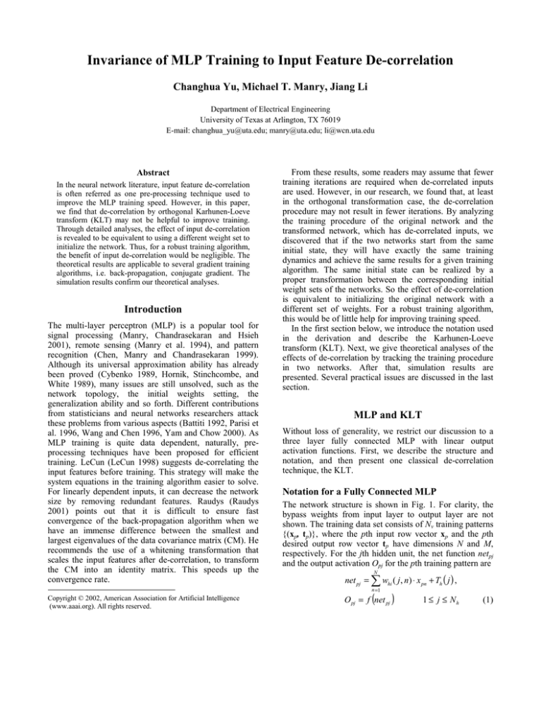
Invariance of MLP Training to Input Feature De-correlation
Changhua Yu, Michael T. Manry, Jiang Li
Department of Electrical Engineering
University of Texas at Arlington, TX 76019
E-mail: changhua_yu@uta.edu; manry@uta.edu; li@wcn.uta.edu
Abstract
In the neural network literature, input feature de-correlation
is often referred as one pre-processing technique used to
improve the MLP training speed. However, in this paper,
we find that de-correlation by orthogonal Karhunen-Loeve
transform (KLT) may not be helpful to improve training.
Through detailed analyses, the effect of input de-correlation
is revealed to be equivalent to using a different weight set to
initialize the network. Thus, for a robust training algorithm,
the benefit of input de-correlation would be negligible. The
theoretical results are applicable to several gradient training
algorithms, i.e. back-propagation, conjugate gradient. The
simulation results confirm our theoretical analyses.
Introduction
The multi-layer perceptron (MLP) is a popular tool for
signal processing (Manry, Chandrasekaran and Hsieh
2001), remote sensing (Manry et al. 1994), and pattern
recognition (Chen, Manry and Chandrasekaran 1999).
Although its universal approximation ability has already
been proved (Cybenko 1989, Hornik, Stinchcombe, and
White 1989), many issues are still unsolved, such as the
network topology, the initial weights setting, the
generalization ability and so forth. Different contributions
from statisticians and neural networks researchers attack
these problems from various aspects (Battiti 1992, Parisi et
al. 1996, Wang and Chen 1996, Yam and Chow 2000). As
MLP training is quite data dependent, naturally, preprocessing techniques have been proposed for efficient
training. LeCun (LeCun 1998) suggests de-correlating the
input features before training. This strategy will make the
system equations in the training algorithm easier to solve.
For linearly dependent inputs, it can decrease the network
size by removing redundant features. Raudys (Raudys
2001) points out that it is difficult to ensure fast
convergence of the back-propagation algorithm when we
have an immense difference between the smallest and
largest eigenvalues of the data covariance matrix (CM). He
recommends the use of a whitening transformation that
scales the input features after de-correlation, to transform
the CM into an identity matrix. This speeds up the
convergence rate.
From these results, some readers may assume that fewer
training iterations are required when de-correlated inputs
are used. However, in our research, we found that, at least
in the orthogonal transformation case, the de-correlation
procedure may not result in fewer iterations. By analyzing
the training procedure of the original network and the
transformed network, which has de-correlated inputs, we
discovered that if the two networks start from the same
initial state, they will have exactly the same training
dynamics and achieve the same results for a given training
algorithm. The same initial state can be realized by a
proper transformation between the corresponding initial
weight sets of the networks. So the effect of de-correlation
is equivalent to initializing the original network with a
different set of weights. For a robust training algorithm,
this would be of little help for improving training speed.
In the first section below, we introduce the notation used
in the derivation and describe the Karhunen-Loeve
transform (KLT). Next, we give theoretical analyses of the
effects of de-correlation by tracking the training procedure
in two networks. After that, simulation results are
presented. Several practical issues are discussed in the last
section.
MLP and KLT
Without loss of generality, we restrict our discussion to a
three layer fully connected MLP with linear output
activation functions. First, we describe the structure and
notation, and then present one classical de-correlation
technique, the KLT.
Notation for a Fully Connected MLP
The network structure is shown in Fig. 1. For clarity, the
bypass weights from input layer to output layer are not
shown. The training data set consists of Nv training patterns
{(xp, tp)}, where the pth input row vector xp and the pth
desired output row vector tp have dimensions N and M,
respectively. For the jth hidden unit, the net function netpj
and the output activation Opj for the pth training pattern are
N
net pj = ∑ whi ( j , n) ⋅ x pn + Th ( j ) ,
n =1
Copyright © 2002, American Association for Artificial Intelligence
(www.aaai.org). All rights reserved.
(
O pj = f net pj
)
1 ≤ j ≤ Nh
(1)
Op1
mx =
x p1
yp1
xp2
yp2
xp 3
yp3
Cx =
1
Nv
ypM
OP,Nh
Fig. 1 MLP network structure
Here xpn denotes the nth element of xp, whi(j, n) denotes the
weight connecting the nth input unit to the jth hidden unit,
Th(j) is the hidden unit threshold and Nh is the number of
hidden units. The activation function f is the sigmoid
function
1
(2)
f net pj =
− net
1 + e pj
The kth output ypk for the pth training pattern is
(
)
N
Nh
n =1
j =1
y pk = ∑ woi (k , n ) ⋅ x pn + ∑ woh (k , j )⋅ O pj + To (k )
(3)
k=1, …, M, where woi(k, n) denotes the weight connecting
the nth input node to the kth output unit, To(k) is the output
threshold and woh(k, j) denotes the weight connecting the
jth hidden unit to the kth output unit. In batch mode
training, the overall performance of a feed-forward
network, can be measured by the mean square error (MSE)
E=
1
Nv
Nv
∑ ∑ [t
2
M
pm
− y pm
p =1 m =1
]
(4)
1 N
T
=
∑ tp −yp ⋅ tp −yp
N v p =1
where tpm denotes the mth element of the pth desired output
vector. Recall that tp and yp are row vectors.
v
(
)(
)
Karhunen-Loeve Transform (KLT)
The KL transform was originally introduced by Karhunen
and Loeve. Here, the orthogonal KLT matrix A is used to
de-correlate the original input feature vector xp to zp:
a12 L a1, N   x p1 
 z p1 
 a11

z 

a
 p 2  = z T = Ax T =  21 a 22 L a 2, N   x p 2  (5)
P
p
 M 
 M
M
M
M  M 





a N ,1 a N , 2 L a N , N   x pN 
 z pN 
For the original training patterns, the mean vector and CM
are
Nv
xp
∑
p 1
(6)
=
[(x p − m x )T (x p − m x )]
∑
p 1
Nv
(7)
=
After applying the KLT, the mean vector and CM of the
de-correlated inputs are
1 Nv
(8)
mz =
∑ z p = m x ⋅ AT
N v p =1
Cz =
xp,N+1
1
Nv
1
Nv
∑ [(z
Nv
p
−mz
p =1
) (z
T
p
−mz
)]
(9)
T
= AC x A
The new CM Cz is a diagonal matrix. The orthogonal KLT
matrix A can be found by the singular value decomposition
(SVD).
Input De-correlation and MLP Training
The effect of de-correlating the input features is analyzed in
this section. We demonstrate our analyses using the full
conjugate gradient algorithm (FCG) (Fletch 1987, Kim
2003).
Assume that two MLP networks are respectively trained
N
N
with training data x p , t p p =v 1 and z p , t p p =v 1 . The
{
}
{
}
networks are said to be equivalent if their hidden layer
activations are identical and their output vectors are
identical for every training pattern.
First, the conditions for ensuring equivalent states in the
two networks are derived. Then we briefly describe the
FCG algorithm. Finally, by induction, we show that the
training dynamics in the two networks are exactly the same.
We will use u to denote the weights in the transformed
network and add an extra subscript ‘d’, representing decorrelation, to other notation for discrimination.
Conditions for Equivalent States
If the weights of the transformed network are uoi, uoh, and
uhi, the thresholds are Tdo, Tdh, then the hidden layer net
functions and network outputs are:
net Tdp = u hi ⋅ z Tp + Tdh = u hi ⋅ A ⋅ x Tp + Tdh
(10)
y Tdp = u oi ⋅ z Tp + Tdo + u oh ⋅ O Tdp
(11)
= u oi ⋅ A ⋅ x Tp + Tdo + u oh ⋅ O Tdp
where the hidden layer output vector Odp is calculated by
applying the sigmoid function to netdp.
From equations (10) and (11), we can see that, if the
weights and thresholds in the original network satisfy:
w hi = u hi ⋅ A , w oi = u oi ⋅ A
(12)
w oh = u oh , To = Tdo , Th = Tdh
(13)
then the two networks will have the same net functions and
outputs, and consequently, the same states. After
initializing the two networks with the strategy in (12) and
(13), they start from the same initial state.
g dhi
The Full Conjugate Gradient Algorithm
In FCG (Fletch 1987, Kim 2003), for the kth training
iteration, the weights and thresholds are updated in
corresponding conjugate directions, P, i.e., in the
transformed network
u oi ← u oi + B 2 ⋅ Pdoi (k ) , u hi ← u hi + B 2 ⋅ Pdhi (k ) (14)
u oh ← u oh + B 2 ⋅ Pdoh (k ) , Tdo ← Tdo + B 2 ⋅ Pdo (k )
Tdh ← Tdh + B 2 ⋅ Pdh (k )
(15)
The weights and thresholds in the original network are
updated in the same way. So, if the two networks have the
same learning factors B2 and the conjugate directions P
satisfy:
Phi = Pdhi ⋅ A , Poi = Pdoi ⋅ A
(16)
Poh = Pdoh , Po = Pdo , Ph = Pdh
(17)
then they will still have the same states as long as they have
the same states in the (k-1)th iteration. It is easy to verify
this because updating the weights and thresholds in (14) to
(17) will ensure conditions (12) and (13).
In FCG, the conjugate directions evolve from iteration to
iteration in the following way:
P (k ) = −g(k ) + B1 P(k − 1)
(18)
Here g is the gradient matrix for the weights and
thresholds. In the transformed network, for certain training
iterations, the gradient matrix of uoi has the form:
∂E

 ∂E
 ∂u (1,1) L ∂u (1, N ) 
oi
oi


∂E
M
M
M
g doi =
=

∂u oi  ∂E
∂E

L
 ∂u oi (M ,1)
∂u oi (M , N )




L
e
z
e
z
⋅
⋅
dp1
p1
dp1
pN
−2 N 

M
M
M
(19)
=
⋅∑ 

N v p =1
e dpM ⋅ z p1 L e dpM ⋅ z pN 


 e dp1 

− 2  N
−2 N 

M ⋅z p =
=
e dp ⋅ x p  ⋅ A T
∑
∑


N v  p =1
N v p =1

e dpM 


where
e dpm = t pm − y dpm
m = 1, L M
(20)
Similarly, the gradient matrix of uoh is:
−2 N
(21)
g doh =
∑ e dp ⋅ O dp
N v p =1
v
v
v
v
The gradient matrix of Tdo is:
− 2 Nv
g do =
∑ e dp
N v p =1
For the hidden weights uhi, the gradient matrix is:
(22)
∂E

 ∂E
 ∂u (1,1) L ∂u (1, N ) 
hi
hi

∂E 
M
M
M
=
=

∂u hi  ∂E
∂E

L
 ∂uhi (N h ,1)
∂uhi (N h , N ) 



 M
M
∂ydpm 
∂y 
 z p1 L  ∑ edpm dpm  z pN 
  ∑ edpm
 m =1
∂Odp1 
∂Odp1 

  m =1

− 2 Nv  

M
M
M
=
∑

N v p =1  M
M



y
y
∂
∂
dpm 
dpm 

 e

L
z
e
z
∑
dpm
p1
dpm
pN




 ∑
O
O
∂
∂
m =1
dpN h 
dpN h 
 m =1


M
 
 
  ∑ edpmuoh (m,1) 
 

− 2  Nv
− 2 N v   m =1
 ∑ Ddp x p  ⋅ AT
M
=
⋅zp =

∑


M
N v p =1 
N v  p =1




(
)
e
u
m
N
,
 ∑ dpm oh
h 

 m =1
(23)
Similarly, the gradient matrix for the hidden unit threshold
vector Tdh:
− 2 Nv
(24)
g dh =
∑ D dp
N v p =1
Applying similar analyses to the original network, we can
write the corresponding gradient matrices:
− 2 Nv
− 2 Nv
g oi =
e p ⋅ x p , g hi =
∑
∑ D p ⋅ x p (25)
N v p =1
N v p =1
g oh =
− 2 Nv
− 2 Nv
− 2 Nv
e p ⋅O p , go =
e p , gh =
∑Dp
∑
∑
N v p =1
N v p =1
N v p =1
(26)
B1 in (18) is the ratio of the gradient energies between the
current iteration and the previous iteration:
g(i )
(27)
B1 =
g(i − 1)
Dynamics of the Training Procedure
In the following, we show by induction that the above two
networks have the same dynamics for full conjugate
gradient training.
In the first training iteration, for both networks,
g d (0) = g(0) = 0 , Pd (0) = P (0) = 0
(28)
In order to calculate B1, we just set
g d (0) = g(0) = 1
(29)
Due to the initialization strategy, at the beginning of the
first iteration, we have
y dp = y p , e dp = e p , O dp = O p , D dp = D p (30)
By observing the gradient matrices (19) to (26), it is
obvious that during the first training iteration, the gradients
in the two networks satisfy
g doi = g oi ⋅ A T , g dhi = g hi ⋅ A T
(31)
g doh = g oh , g do = g o , g dh = g h
(32)
Then the energy of gradients in the transformed network
for the first training iteration is:
j =1
T
j =1
j)
j)
+ ∑ g (doh
⋅ g (doh
j =1
(
T
( j)
T
j =1
( j)
⋅ g do + (g dh ) ⋅ g dh
Nh
) +∑g
T T
T
( j)
hi
(
T
T
T
o
( j)
A ⋅ g hi A
j =1
( ) + (g )
+ ∑ g (ohj ) ⋅ g (ohj )
j =1
T
do
= ∑ g oi A ⋅ g oi A
M
The derivation for the (n+1)th iteration is similar to the
analyses in the first iteration. From (30), conditions (31)
and (32) are met again. Just as in (33), we have
g d (n + 1) = g(n + 1)
(38)
j T
dhi
j
dhi
( ) + (g )
M
M
Nh
( ) + ∑ g ( ) ⋅ (g ( ) )
M
( j)
g d (1) = ∑ g (doij ) ⋅ g doi
)
T T
⋅ g o + (g h ) ⋅ g h
T
= g(1)
(33)
where superscript (j) denote the jth row vector in the
corresponding matrix. From equation (27), (29) and (33),
we conclude that B1 is the same in the two networks. Based
on equations (28), (31), (32), and substituting them into
(18), the new conjugate directions in the first training
iteration satisfy conditions (16) and (17).
In order to prove that the two networks have same state
after the first training iteration, we still need to verify that
the learning factor B2 is the same in the two networks. The
learning factor B2 is found by solving:
∂E
=0
(34)
∂B 2
In the transformed network, the output vector after a
training iteration is:
y Tdp = (u oi + B 2 Pdoi ) ⋅ z Tp + (Tdo + B 2 Pdo )Tdo
(
)
+ (u oh + B 2 Pdoh ) ⋅ f (u hi + B 2 Pdhi ) ⋅ z Tp + (Tdh + B 2 Pdh )
(35)
where f denotes the vector form of the sigmoid function.
The current weights and thresholds satisfy conditions (12),
(13), and the updating directions satisfy (16) and (17), thus
equation (35) can be expressed as:
y Tdp = (w oi + B 2 Poi )A T ⋅ Ax Tp + (To + B 2 Po )
(
weights and thresholds satisfy conditions (12) and (13), so
(33) becomes
g d (n ) = g(n )
(37)
)
+ (w oh + B 2 Poh )f (w hi + B 2 Phi )A T Ax Tp + (Th + B 2 Ph )
= y Tp
(36)
Hence after the first training iteration, the outputs in the
two networks are exactly the same. Substituting them into
(4) will result in the same expression for E in the two
networks. Thus any practical methods for solving (34) will
yield the same B2 for the two networks.
From the above analyses, it is clear that the two networks
will have exactly the same state after the first training
iteration.
We assume for the nth iteration, that the two networks
still reach the same state after training. This implies that in
the (n+1)th iteration, equation (30) is satisfied, current
So once again B1 is the same in the two networks. Using
this result, combined with equations (18), (31) and (32), it
is easy to show that conditions (16) and (17) are valid in
the (n+1)th iteration. As equation (35) is true for an
arbitrary iteration, from conditions (16), (17), (12) and
(13), equation (36) is satisfied in the (n+1)th iteration.
Based on exactly the same reason as in the first iteration, B2
will be same in the two networks. As a result, conditions
(12) and (13) are proved to be true for the new updated
weights and thresholds after the (n+1)th training iteration.
That is to say, the two networks will still have same state
after the (n+1)th training iteration.
From the above induction, the training dynamics of the
two networks are proved to be exactly the same. Actually,
for other gradient-related algorithms, i.e. output weight
optimization-backpropagation (OWO-BP), output weight
optimization-hidden weight optimization (OWO-HWO),
we can prove similar conclusions as long as learning
factors are optimal, meaning that equation (34) is satisfied.
Without the sufficient condition of equation (34), the
training errors of two equivalent networks may diverge
during training.
Simulation
The results in the last section are verified using four
training data sets. Our simulations were carried out on a
733Mhz Pentium III, running Windows 2000 and using the
Visual C++ 6.0 compiler.
Training data set Twod.tra contains simulated data based
on models from backscattering measurements. This training
file is used in the task of inverting the surface scattering
parameters from an inhomogeneous layer above a
homogeneous half space, where both interfaces are
randomly rough. The parameters to be inverted are the
effective permittivity of the surface, the normalized rms
height, the normalized surface correlation length, the
optical depth, and single scattering albedo of an inhomogeneous irregular layer above a homogeneous half
space from back scattering measurements.
The data set has 8 inputs, 7 outputs, and 1768 patterns.
We use 10 hidden units in a three-layer MLP. The
networks are trained using FCG for 200 iterations. From
the simulation results of figure 2, it is clear that the two
networks have exactly the same dynamics.
Training data set mattrn.dat provides the data for
inversion of random two-by-two matrices. Each of the 2000
patterns consists of 4 input features and 4 output features.
The input features, which are uniformly distributed
between 0 and 1, represent matrix elements and the four
Simulation results for example Data: Twod.tra, Structure: 8-10-7
Simulation results for example Data: fmtrain.dat, Structure: 5-10-1
0.14
Original dat a
0.325
Original data
KLT data
0.32
KLT data
0.12
0.315
0.1
MSE
MSE
0.31
0.305
0.06
0.3
0.295
0.04
0.29
0.02
0.285
0
20
40
60
80
100
120
Training iterations
140
160
180
0
200
Fig. 2 Simulation results for example 1 data: Twod.tra,
Structure: 8-10-7
0
20
40
60
80
100 120 140
Training iterations
160
180
200
Fig. 4 Simulation results for example 3 data: fmtrain.dat,
Structure: 5-10-1
Simulation results for example Data: single2.tra, Structure: 16-20-3
2.6
Simulation results for example Data: mattrn.dat, Structure: 4-10-4
0.14
Original data
KLT data
Original data
KLT data
2.4
0.12
2.2
MSE
0.1
MSE
0.08
0.08
2
1.8
0.06
1.6
0.04
0.02
1.4
0
20
40
60
80
100
120
Training iterations
140
160
180
200
Fig. 3 Simulation results for example 2 data: mattrn.dat,
Structure: 4-10-4
output features are elements of the corresponding inverse
matrix. The determinants of the input matrices are
constrained to be between 0.3 and 2.
We chose the MLP structure 4-10-4 and trained the
networks for 200 iterations. The simulation results of figure
3 show the same dynamics for the two networks.
Training data fmtrain.dat is used to train a neural
network to perform demodulation of an FM (frequency
modulation) signal containing a sinusoidal message. It has
5 inputs, 1 output, and 1024 patterns. The data are
generated from the equation
r(n) = Camp • cos[2π • n • Cfreq + Mamp
• sin(2π • n • Mfreq )]
where Camp is the Carrier Amplitude, Mamp is the
Message Amplitude, Cfreq is the normalized Carrier
frequency, Mfreq is the normalized message frequency. In
this data set, Camp = .5, Cfreq = .1012878, Mfreq =
.01106328, and Mamp=5. The five inputs are r(n-2), r(n-1),
r(n), r(n+1), and r(n+2). The desired output is cos(2π • n •
Mfreq ). In each consecutive pattern, n is incremented by 1.
1.2
0
20
40
60
80 100 120 140
Training iterations
160
180
200
Fig. 5 Simulation results for example 4 data:Single2.tra,
Structure: 16-20-3
We use 10 hidden units in the three-layer MLP. The
networks are trained using FCG for 200 iterations. Figure 4
shows the result.
Single2.tra consists of 16 inputs, 3 outputs and 5992
patterns. It represents the training set for inversion of
surface permittivity, the normalized surface rms roughness,
and the surface correlation length found in the back
scattering models from randomly rough dielectric surfaces.
The first 16 inputs represent the simulated back
scattering coefficient measured at 10, 30, 50 and 70
degrees at both vertical and horizontal polarization. The
remaining 8 are various combinations of ratios of the
original eight values. These ratios correspond to those used
in several empirical retrieval algorithms (Fung, Li and
Chen 1992).
We chose the MLP structure 16-20-3 and trained the
networks for 200 iterations. From the simulation results of
figure 5, we can see that there are obvious differences
between the two curves. This phenomenon is caused by
problems in the matrix A. For data sets Twod.tra,
mattrn.dat, and fmtrain.dat, we found that A calculated by
the SVD is orthogonal, i.e. ATA = I, so the analyses in the
last section are satisfied. However, for the training data file
Single2.tra, A is not orthogonal because of problems in the
SVD. Our analyses are not valid for this case and the two
networks are not equivalent, as seen in figure 5.
Conclusion
In this paper, we analyzed the effect of orthogonally
transformed input vectors on MLP training. Using the
concept of equivalent states, we have shown that this decorrelation procedure has no effect on the error per
iteration for the FCG training algorithm. Of course, decorrelation is still useful for compression purposes and as a
means for reducing the number of operations per iteration
in some training algorithms. We have derived our results
for networks that have bypass weights. These results are
still valid when the bypass weights are set to zero, or
equivalently, removed.
Although the analyses in this paper are based upon FCG,
they apply equally well to BP, and other gradient-based
training algorithms when optimal learning factors are used.
Acknowledgement
This work was supported by the Advanced Technology
Program of the state of Texas, under grant number 0036560129-2001.
References
Battiti, R. 1992. First- and Second-order Methods for
Learning: between Steepest Descent and Newton’s Method.
Neural Computation 4 (2): 141-166.
Chen, H. H.; Manry, M. T.; and Chandrasekaran, H. 1999.
A Neural Network Training Algorithm Utilizing Multiple
Sets of Linear Equations. Neurocomputing 25: 55-72.
Cybenko, G. 1989. Approximation by superpositions of a
sigmoidal function. Mathematics of Control, Signals, and
Systems 2: 303-314.
Fletch, R. 1987. Practical Methods of Optimization. John
Wiley & Sons.
Fung, A.K.; Li, Z.; and Chen, K.S. 1992. Back Scattering
from a Randomly Rough Dielectric Surface. IEEE
Transactions on Geoscience and Remote Sensing 30 (2):
356-369.
Hornik, K.; Stinchcombe, M.; and White, H. 1989.
Multilayer
feedforward
networks
are
universal
approximators. Neural Networks 2: 359-366.
Kim, T. H.; Manry, M. T.; and Maldonado, F. J. 2003.
New Learning Factor and Testing Methods for Conjugate
Gradient Training Algorithm. In Proceedings of 2003
International Joint Conference on Neural Networks, 20112016. Portland, OR: International Joint Conference on
Neural Networks.
LeCun Y., et al. 1998. Efficient BackProp. In Orr, G. B.
and Muller, K. R. eds., Neural Networks: Tricks of the
Trade. Springer-Verlag.
Manry, M. T., et al. 1994. Fast Training of Neural
Networks for Remote Sensing. Remote Sensing Reviews 9:
77-96.
Manry, M. T.; Chandrasekaran, H.; and Hsieh, C. H. 2001.
Signal Processing Using the Multiplayer Perceptron. CRC
Press.
Parisi, R.; Claudio, E. D.; Orlandi G.; and Rao B. D. 1996.
A Generalized Learning Paradigm Exploiting the Structure
of Feedforward Neural Networks. IEEE Transactions on
Neural Networks 7 (6): 1450-1460.
Raudys, Š. 2001. Statistical and Neural Classifiers: An
Integrated Approach to Design. Springer-Verlag.
Wang, G. J., and Chen C. C. 1996. A Fast Multilayer
Neural-network Training Algorithm Based on the Layerby-layer Optimizing Procedures. IEEE Transactions on
Neural Networks 7 (3): 768-775.
Yam, Y. F., and Chow, W. S. 2000. A Weight Initialization
Method for Improving Training Speed in Feedforward
Neural Network. Neurocomputing 30: 219-232.