Real-Time Simulation of Herds Moving Over Terrain
Joel Gompert
Constraint Systems Laboratory
University of Nebraska-Lincoln
jgompert@cse.unl.edu
Abstract
We present a method for animating herds of animals to follow terrain surfaces in real time. This method involves making modifications to Reynold’s boids algorithm. The modifications use local properties of the terrain and thus have low
complexity. They produce naturally behaving herds that follow the terrain, swerving around hills and attempting to reduce energy expenditure. The terrain-following rule has a parameter that can be adjusted to produce different behaviors.
Empirical analysis shows how this parameter affects energy
expenditure of the animals while traveling over the terrain.
See demo: http://consystlab.unl.edu/our work/herds.html
Introduction
Reynolds introduced the efficient boids algorithm for animating flocks of animals (1987; 1999), where each animal
makes its own decisions on how to move. Reynolds suggested that further modifications could lead to a herd model
by giving the animals the ability to follow three-dimensional
terrain. This paper explores such modifications. The animals in Reynold’s flocks move according to three simple
rules, each resulting in an acceleration, which are combined
to animate the animals:
1. Separation: accelerating away from nearby members of
the flock that are closer than some threshold distance.
2. Alignment: adjusting an animal’s velocity to match the
average velocity of its neighbors. And
3. Cohesion: accelerating towards the center of the flock.
Additional rules can create new behaviors such as obstacle
avoidance and goal seeking. We first discuss the mapping
from 2D to 3D and the necessary correction for 3D. We then
derive a new rule for traversing terrain.
Moving From Flocks to Herds
In order to traverse terrain, the animals must be constrained
to the terrain’s surface. One possibility is to use 3D flocking and add constraints or forces to keep the animals on the
surface. However we chose to use 2D flocking, and apply a
scaling correction to the movement for the third dimension.
c 2005, American Association for Artificial IntelliCopyright gence (www.aaai.org). All rights reserved.
We denote the 2D flocking space as F. F-vector refers to
a vector in F. Likewise P refers to 3D space. The terrain
is a mapping m : F 7→ P. We compute the flocking animation in F, and render the animals at their corresponding
location in P. We assume there is an ‘up’ direction in P dictated by gravity, and h(p ∈ F) gives the P-coordinate along
that axis.1 The gradient ~g (p) of h(p) is a vector whose components are partial derivatives of h evaluated at the point
∂h ∂h T
p (e.g., ~g(x, y) = [ ∂x
, ∂y ] ). The gradient is a vector
pointing in the direction of the greatest increase of h, and
its magnitude is the slope s(p) = ||~g(p)|| of the terrain in
that direction. The slope in the direction of a vector ~v is
·~
g (p)
. The gradient at a point can be efficiently
s~v (p) = ~v||~
v ||
computed for most terrain models.
3D Correction
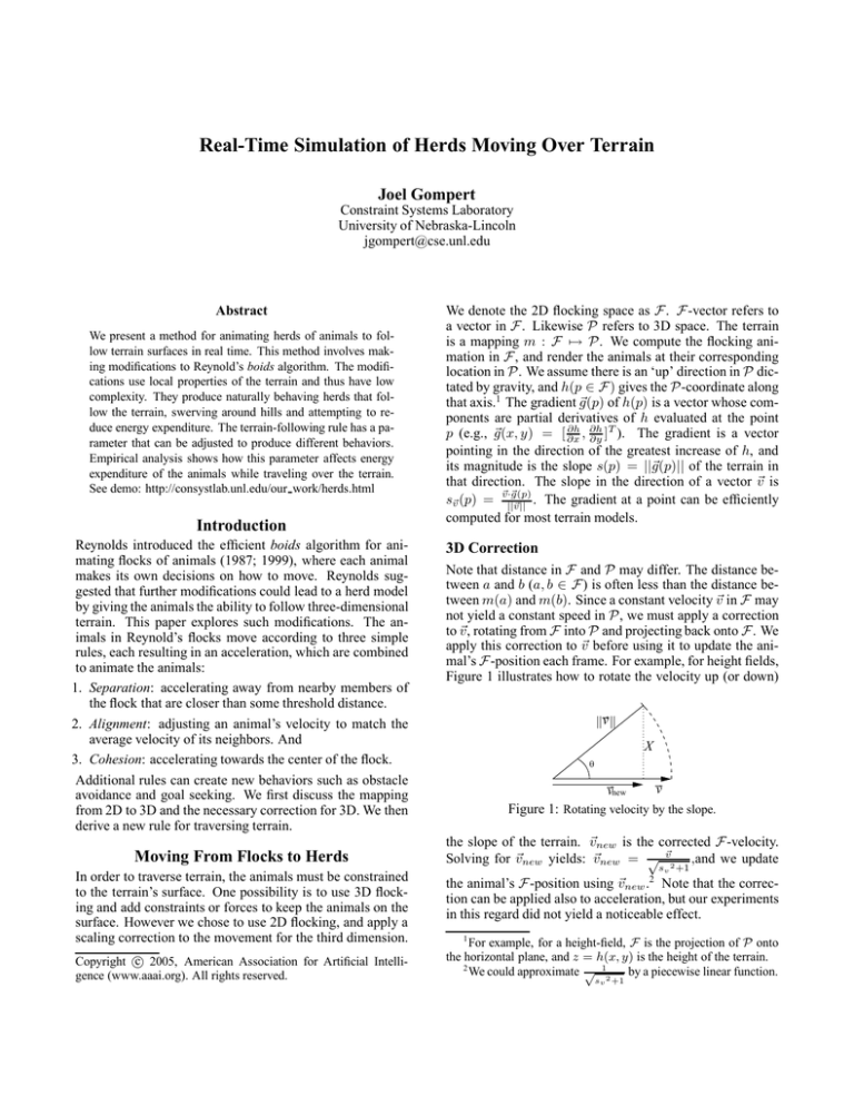
Note that distance in F and P may differ. The distance between a and b (a, b ∈ F) is often less than the distance between m(a) and m(b). Since a constant velocity ~v in F may
not yield a constant speed in P, we must apply a correction
to ~v , rotating from F into P and projecting back onto F. We
apply this correction to ~v before using it to update the animal’s F-position each frame. For example, for height fields,
Figure 1 illustrates how to rotate the velocity up (or down)
|| v ||
X
θ
v
vnew
Figure 1: Rotating velocity by the slope.
the slope of the terrain. ~vnew is the corrected F-velocity.
Solving for ~vnew yields: ~vnew = √ ~v2 ,and we update
sv +1
the animal’s F-position using ~vnew .2 Note that the correction can be applied also to acceleration, but our experiments
in this regard did not yield a noticeable effect.
1
For example, for a height-field, F is the projection of P onto
the horizontal plane, and z = h(x, y) is the height of the terrain.
2
by a piecewise linear function.
We could approximate √ 1
sv 2 +1
Now we have a framework for mapping F to P, but the
herd still travels straight over terrain features in its way, as in
Path 1 in Figure 2. However, we may prefer a more naturalPath 1
Path 2
Path 3
Figure 4. We can now choose K to minimize energy expenditure. Setting K = 0 eliminates the effect. Increasing K
Average Energy Expenditure
Natural Behavior Over 3D Terrain
100
95
90
85
80
75
70
65
0
12.5
25
37.5
50
62.5
75
K
Figure 2: Possible paths to get past a hill.
looking route such as Path 2 or 3.
Rate of energy expenditure
Natural Routes One possibility is to pre-compute a route.
For example, Kapoor describes a method for computing the
geodesic shortest path across the surface of a polygonal
mesh (1999). The shortest path is not necessarily what we
would like. Animals and humans naturally choose behaviors
that minimize energy expenditure. Further, pre-computing
shortest paths violates the essence of the boids algorithm.
Consequently we consider how the terrain affects energy expenditure. (Minetti 1993; Minetti & Alexander 1997) lead
us to form an energy function like Figure 3. Generally, to
Minimum = −0.1
Slope
Figure 3: Energy expenditure as a function of slope.
conserve energy, the herd should try to follow contour lines.
But following a contour line around a wide, short hill might
be less economical than a more direct route.
Terrain Force Our solution is to apply a force that resists
motion orthogonal to the contour lines. We obtain nice results when the force is proportional to the gradient. If the animals are already following a contour line, then we need to
avoid pushing them up or downhill. Thus, the force should
also be proportional to the negative of the component of velocity along the gradient, thus for some constant K:
~ = −Ks ~v · ~g ~g = −K (~v · ~g ) ~g .
F
(1)
||~g||
||~g||2
We define F~ = 0 when ||~g|| = 0. To determine a value
for K we performed experiments with herds of 50 animals
traveling over smooth, randomly-generated terrain from one
location to a goal point. We varied the constant K and calculated an estimate for the average energy expended over 300
trips. We estimated energy expenditure at each time step using the energy function of Figure 3. The results are shown in
Figure 4: Mean energy expenditure as a function of K.
decreases the energy expenditure, up to a point, after which
the animals take longer routes. At some higher value, the
animals can no longer accelerate enough to climb hills, and
may never reach their goal. We can choose K to obtain various behaviors, e.g. cattle may choose to stick close to the
contour lines, while mountain goats may prefer to hop over
the top of a steep hill. These modifications to the flocking algorithm produce pleasing results. The herd curves naturally
along terrain, and can divide into two groups to go opposite
directions around a hill, regrouping on the other side.
Summary
In order to create the behavior of herds moving over terrain
we have made modifications to the basic flocking algorithm:
1. We use a 2D algorithm, mapped into 3D space.
2. At each time step, we update the position of an each animal not by its velocity ~v but by ~v mapped from F to P.
3. We add an additional rule: an acceleration equal to
−K (~v||~·~gg||)~g .
The constant K controls how tightly the herd will follow
the contour lines of the terrain. K can be adjusted for low
energy expenditure or other terrain-following behaviors. In
the future we would like to develop higher-level behaviors
such as migrating, finding food, and avoiding predators.
Acknowledgments
This research is supported by NSF CAREER Award #0133568.
The author is indebted to Christopher Kline for the source to his
boids implementation(2002) and to Ken Bayer for the terrain generation.
References
Kapoor, S. 1999. Efficient computation of geodesic shortest
paths. In ACM Symposium on Theory of Computing.
Kline, C. 2002. web.media.mit.edu/˜ckline/. Cornell University.
Minetti, A., and Alexander, R. M. 1997. A theory of metabolic
costs for bipedal gait. Journal of Theoretical Biology 186:467–
476.
Minetti, A. E. 1993. Mechanical determinants of grade walking
energetics. Journal of Physiology 472:725–735.
Reynolds, C. 1987. Flocks, herds, and schools: A distributed
behavior model. In SIGGRAPH, 25–34.
Reynolds, C. W. 1999. Steering behaviors for autonomous characters. In Game Developers Conference, 763–782.