The Indifferent Naive Bayes Classifier
Jesús Cerquides
Ramon López de Màntaras
cerquide@maia.ub.es
mantaras@iiia.csic.es
Dept. de Matemàtica Aplicada i Anàlisi (MAiA) Institut d’Investigació en Intel.ligència Artificial (IIIA)
Universitat de Barcelona (UB)
Spanish Scientific Research Council (CSIC)
Gran Via, 585
Campus UAB
08007 Barcelona, Spain
08193 Bellaterra, Spain
Abstract
The Naive Bayes classifier is a simple and accurate classifier.
This paper shows that assuming the Naive Bayes classifier
model and applying Bayesian model averaging and the principle of indifference, an equally simple, more accurate and
theoretically well founded classifier can be obtained.
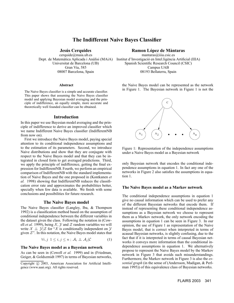
the Naive Bayes model can be represented as the network
in Figure 1. The Bayesian network in Figure 1 is not the
C
Introduction
In this paper we use Bayesian model averaging and the principle of indifference to derive an improved classifier which
we name Indifferent Naive Bayes classifier (IndifferentNB
from now on).
First we introduce the Naive Bayes model, paying special
attention to its conditional independence assumptions and
to the estimation of its parameters. Second, we introduce
Naive distributions and show that they are conjugate with
respect to the Naive Bayes model and that they can be integrated in closed form to get averaged predictions. Third,
we apply the principle of indifference, getting the final expression for IndifferentNB. Fourth, we perform an empirical
comparison of IndifferentNB with the standard implementation of Naive Bayes and the one proposed in (Kontkanen et
al. 1998) showing that IndifferentNB reduces the classification error rate and approximates the probabilities better,
specially when few data is available. We finish with some
conclusions and possibilities for future research.
The Naive Bayes model
The Naive Bayes classifier (Langley, Iba, & Thompson
1992) is a classification method based on the assumption of
conditional independence between the different variables in
the dataset given the class. Following the notation in (Cowell et al. 1999), being X , Y and Z random variables we will
write X ⊥
⊥ Y|Z for “X is conditionally independent on Y
given Z”. In this notation, the Naive Bayes model states that
∀i, j 1 ≤ i, j ≤ n ; Ai ⊥
⊥ Aj |C
(1)
The Naive Bayes model as a Bayesian network
As can be seen in (Cowell et al. 1999) and in (Friedman,
Geiger, & Goldszmidt 1997) in terms of Bayesian networks,
Copyright c 2003, American Association for Artificial Intelligence (www.aaai.org). All rights reserved.
A1
A2
An
Figure 1: Representation of the independence assumptions
under a Naive Bayes model as a Bayesian network
only Bayesian network that encodes the conditional independence assumptions in equation 1. In fact any one of the
networks in Figure 2 also satisfies the assumptions in equation 1.
The Naive Bayes model as a Markov network
The conditional independence assumptions in equation 1
give no causal information which can be used to prefer any
of the different Bayesian networks that encode them. If
instead of representing these conditional independence assumptions as a Bayesian network we choose to represent
them as a Markov network, the only network encoding the
assumptions in equation 1 can be seen in Figure 3. In our
opinion, the use of Figure 1 as representation of the Naive
Bayes model, that is correct when interpreted in terms of
acausal Bayesian networks, is slightly confusing, due to the
fact that if it is interpreted in terms of causal Bayesian networks it conveys more information than the conditional independence assumptions in equation 1. We alternatively
propose to represent the Naive Bayes model by the Markov
network in Figure 3 that avoids such misunderstandings.
Furthermore, the Markov network in Figure 3 is also the essential graph (in the sense of (Andersson, Madigan, & Perlman 1995)) of this equivalence class of Bayesian networks.
FLAIRS 2003
341
C
A1
We will note Φ = {φi,v,c |c ∈ C; 1 ≤ i ≤ n; v ∈ Ai }. It
should be noted that αc is introduced only in order to ease
understanding and notation, because it can be determined
given Φ by means of the constraints.
Suppose we need to know the probability of an unclassified observation S being in class SC given a Naive Bayes
model M . Applying the independence assumptions and substituting the parameters we have that
C
A2
A1
An
A2
An
C
p(SC , S|M ) = αSC
n
Y
φi,S
i=1
A1
A2
An
Figure 2: Alternative representations of the independence
assumptions under a Naive Bayes model as a Bayesian network
i ,SC
αSC
(3)
In many cases, the Naive Bayes classifier has suffered
from “the mind projection fallacy”, to use the term introduced by Jaynes in (Jaynes 1996). Hence, it has been
accepted that what we need to do is to approximate αj and
φi,v,j by the frequencies in the data set. Defining NC (c)
as the number of observations in class c in the dataset and
Ni,C (v, c) as the number of observations with class c and
value v for attribute Ai , the maximum likelihood Naive
Bayes approximates αc , φi,v,c as follows:
C
NC (c)
αc = P
NC (c0 )
(4)
c0 ∈C
Ni,C (v, c)
αc
(5)
NC (c)
It has been empirically noticed that approximating these
probabilities by their frequencies in the dataset can lead to a
value of zero in expression (3). This can happen if one of the
φi,Si ,SC is zero, that is if the value of one of the attributes Ai
of the new observation S, that we are trying to classify, has
not been observed in the dataset for the class SC . In other
words, if the number of observations in the dataset fulfilling Ai = Si and C = SC is zero. To avoid this problem,
a “softening” consisting in assigning a small probability instead of zero to φi,Si ,SC can be done. That softening can improve the accuracy of the classifier. A set of ad hoc not well
founded softening methods have been tried (Cestnik 1990;
Kohavi, Becker, & Sommerfield 1997).
In (Kontkanen et al. 1998), Kontkanen et al. propose an
approach for Instance Based Learning (IBL) and apply it to
the Naive Bayes classifier. This approach is based on the
Bayesian model averaging principle (Hoeting et al. 1998).
They accept the Bayesian network in Figure 1 plus an assumption equivalent to the Dirichlet assumption as appears
in (Heckerman, Geiger, & Chickering 1995). More conφ
cretely, they define θi,v,c = i,v,c
and arrive to the conαc
clusion that if we accept a Dirichlet prior for α. and for
each θi,.,c , that is if (α1 , . . . , α#C ) ∼ Di(µ1 , . . . , µ#C )
and (θi,1,c , . . . , θi,#Ai ,c ) ∼ Di(σi,1,c , . . . , σi,#Ai ,c ) where
µc , σi,v,c are the prior hyperparameters, then the classifier
resulting from applying Bayesian model averaging can be
represented as a Naive Bayes with the following softened
approximation of αc , φi,v,c (Kontkanen et al. 1998):
φi,v,c =
A1
An
A2
Figure 3: Representation of the independence assumptions
under a Naive Bayes model as a the Markov network
Naive Bayes parameters
Let C be the class attribute, V = {A1 , . . . , An } the set
of attributes and C,Ai random variables over C,Ai respectively. Under the multinomial assumption (see (Heckerman,
Geiger, & Chickering 1995)), a Naive Bayes model M can
be characterized by the following assumptions, parameters
and constraints:
• The conditional independence assumptions in Equation 1.
• For each class c ∈ C:
– The model has a parameter αc = P (C = c|M ).
– For each attribute Ai , 1 ≤ i ≤ n:
∗ The model includes a set of parameters
φi,v,c = P (Ai = v ∧ C = c|M )
one for each possible value v ∈ Ai .
∗ The
P model includes the constraint that αc
φi,v,c .
(2)
=
v∈Ai
• The model includes the constraint that
P
αc = 1.
c∈C
From now on we will use the term Naive Bayes model to
refer to this set of assumptions, parameters and constraints.
342
FLAIRS 2003
αc = P
NC (c) + µc
(NC (c0 ) + µc0 )
c0 ∈C
(6)
φi,v,c =
Ni,C (v, c) + σi,v,c
P
αc
NC (c) +
σi,v0 ,c
(7)
v 0 ∈Ai
Kontkanen’s work sheds some light on why “softening” improves accuracy and shows that accuracy can be further improved if the “softening” has a theoretically well founded
basis.
In spite of pointing in the right direction, in our opinion,
Kontkanen et al. disregard the fact that the application of
the Dirichlet assumption assumes a certain causal meaning
in the direction of the edges in a Bayesian network. In fact,
applying the same assumption to any of the Bayesian networks in Figure 2, which encode the same set of conditional
independences, will provide a different result. In addition to
that, the situation allows for the application of the principle
of indifference. First enunciated by Bernoulli and afterwards
advocated for by Laplace, Jaynes and many others (Jaynes
1996), the principle of indifference, also known as the principle of insufficient reason tell us that if we are faced with
a set of exhaustive, mutually exclusive alternatives and have
no significant information that allow us to differentiate any
one of them, we should assign all of them the same probability. As has been demonstrated in (Jaynes 1996) and in
(Bernardo 2003), the principle of indifference can be seen as
a special case of the more general objective Bayesian techniques of maximum entropy and reference analysis.
In the following section we show that accepting the Naive
Bayes model as defined above, it is possible to find a family
of probability distributions that is conjugate to the model and
that allows for a closed calculation of the Bayesian model
averaging. After that we see that the principle of indifference suggests that the prior to be used is in this family of
distributions. We will see that under this setting an additional relationship between the hyperparameters appears that
has not been noticed in (Kontkanen et al. 1998).
Naive distributions
Naive distributions are probability distributions over the set
of Naive Bayes models with two main characteristics:
• They allow for the tractable averaging of Naive Bayes
models in order to compute the probability of an unseen
example.
• They are conjugate to the Naive Bayes model, hence allowing to be learnt from data.
A Naive distribution over a classified discrete domain ΩC
0
is defined by a hyperparameter set N0 = {Ni,C
(v, c)|1 ≤
i ≤ n; v ∈ Ai ; c ∈ C} that fulfills the following condition:
Defining NC0 (c) as
X
0
N0,C
(v, c)
(8)
NC0 (c) =
v∈A0
0
N should fulfill
∀i NC0 (c) =
X
0
Ni,C
(v, c)
(9)
v∈Ai
We will say that P (M |ξ) follows a Naive distribution with
hyperparameter set N0 iff the probability for a concrete
Naive Bayes model is given by
0
Ni,C
n Y (v,c)
Y
φv,i,c
αc
i=1 v∈Ai
c∈C
(10)
where K is a normalization constant.
Naive distributions are a hyper Markov law in the sense
of (Dawid & Lauritzen 1993), for the Markov network in
Figure 3. The proofs for the following results can be found
in (Cerquides & López de Màntaras 2003).
P (M |ξ) = K
Y
0
αc NC (c)
Calculating probabilities with Naive distributions
Assume that our data is generated by a Naive Bayes model
and that P (M |ξ) follows a Naive distribution with hyperparameter set N0 . We can calculate the probability of an observation S, SC given ξ by averaging over the set of Naive
Bayes models
Z
P (S, SC |ξ) =
P (S, SC |M )P (M |ξ)
(11)
M ∈M
Solving the integral we have that
P (SC |S, ξ) = K00
NC0 (SC ) + 1 +
n
X
#Ai − n ×
i=1
×
!
n
0
Y
Ni,C
(Si , SC ) + 1
i=1
NC0 (SC ) + #Ai
(12)
where K00 is a normalization constant and #Ai is the number
of possible values for attribute Ai
Learning with Naive distributions
Given that our data is generated by a Naive Bayes model,
that P (M |ξ) follows a Naive distribution with hyperparameter set N0 and that D is a dataset containing independent
identically distibuted complete observations over a classified discrete doman ΩC , the posterior probability over models given D and ξ ,P (M |D, ξ), follows a Naive distribution
with hyperparameter set N0∗ where:
0∗
0
(v, c) = Ni,C (v, c) + Ni,C
(v, c)
Ni,C
(13)
The Indifferent Naive Bayes Classifier
In the case of Naive Bayes models, the principle of indifference tells us that, in the lack of better information, we should
assign an equal probability to every Naive Bayes model, that
is
∀M ∈ M p(M |I) = Q
(14)
where Q is a constant. Analyzing equation 10, we can see
that a Naive distribution having
0
N0 = {Ni,C
(v, c) = 0|1 ≤ i ≤ n; v ∈ Ai ; c ∈ C}
(15)
assigns an equal probability to every Naive Bayes model.
The Indifferent Naive Bayes classifier is defined by accepting the prior probability distribution over the set of models to follow a Naive distribution with parameter set N0
given by equation 15, using the formerly presented results
FLAIRS 2003
343
to calculate the Naive posterior probability distribution over
models and to calculate probabilities for examples given that
the posterior is a Naive distribution.
It is easy to see that the classifier can be represented by a
Naive Bayes model that uses the following softened approximations:
n
P
NC (c) + 1 +
#Ai − n
i=1
αc = P
(16)
n
P
0
(NC (c ) + 1 +
#Ai − n)
i=1
c0 ∈C
Ni,C (v, c) + 1
αc
(17)
φi,v,c =
NC (c) + #Ai
Comparing these results with the ones from (Kontkanen et
al. 1998) shown in equations 6 and 7 it is worth noticing the
following two facts:
• In (Kontkanen et al. 1998), Kontkanen et al. assume a
Dirichlet prior distribution with a set of hyperparameters
that have to be fixed at some point in time. This means
that a methodologic usage of that classifier requires an assessment of the prior hyperparameters for each dataset in
which we would like to apply it. Instead, we have used the
principle of indifference to obtain a prior without information about the dataset besides the number of attributes
and the cardinality of its attributes and class.
• In equations 6 and 7 the hyperparameters µ. and σi,.,c ,
for α. and θi,.,c are not related. Instead, in our approach
there is a link between the softening parameters, because
the value of αc in equation 16, depends not only on the
number of classes but also on the number of attributes,
n, and on the number of values of each attributes, #Ai ,
and the value of φi,v,c in equation 17, depends also on the
number of values of the attribute, #Ai .
Furthermore, assuming a Naive distribution is compatible
with any of the different Bayesian networks encoding the
independence assumptions in a Naive Bayes model and provides the same result for all of them, because no additional
causal information is assumed from the direction of the
edges in the network. The experimental results in the next
section show that these facts lead to a reduced error rate of
the classifier.
Dataset
Attributes
Instances
Classes
Missing
5
14
10
6
36
13
15
10
4
16
22
8
64
8
35
16
3781
48842
699
1728
3196
303
690
214
150
20000
8124
12960
5620
768
316
435
15
2
2
4
2
2
2
2
3
26
2
5
10
2
19
2
few
some
16
no
no
some
few
none
none
none
some
no
none
no
some
few
DC REDITS
ADULT
BREAST
CAR
CHESS
CLEVE
CRX
GLASS
IRIS
LETTER
MUSHROOM
NURSERY
OPTDIGITS
PIMA
SOYBEAN
VOTES
Table 1: Datasets information
We used cross validation, and we made two experiments:
taking all of the learning fold and taking only 10 % of it.
This is done because the three methods converge to the same
model given enough data. Hence, comparing them when the
size of the training data is small can provide us with good
insight of how they differentiate. The classifiers compared
were:
• MAPNB: The standard Naive Bayes algorithm using frequencies as probability estimates, as shown in equations
4 and 5.
• BIBL: The algorithm appearing in (Kontkanen et al.
1998) and shown in equations 6 and 7 and fixing the hyperparameters to get uniform prior probability distributions.
• IndifferentNB: Our Indifferent Naive Bayes as described
in equations 16 and 17.
Experimental results
We tested three algorithms over 15 datasets from the Irvine
repository (Blake, Keogh, & Merz 1998) plus our own credit
screening database. The dataset characteristics are described
in Table 1.
To discretize continuous attributes we used equal frequency
discretization with 5 intervals. For each dataset and algorithm we tested both accuracy and LogScore. LogScore is
calculated by adding the minus logarithm of the probability assigned by the classifier to the correct class and gives
an idea of how well the classifier is estimating probabilities
(the smaller the score the better the result). If we name our
test set D0 we have
X
− log(P (SC |S, M )) (18)
LogScore(M, D 0 ) =
(S,SC
344
FLAIRS 2003
)∈D 0
(a) Error rate
(b) Log score
Figure 4: Comparison of IndifferentNB and BIBL using
10% training data
The detailed experimental results can be found in
(Cerquides & López de Màntaras 2003). Here we will only
summarize the most important points.
IndifferentNB against BIBL In order to compare the accuracy and LogScore of IndifferentNB and BIBL we have
References
(a) Error rate
(b) Log score
Figure 5: Comparison of IndifferentNB and MAPNB using
10% training data
drawn two graphs, comparing both scores using 10% of the
training data.
• In Figure 4(a) we can see that accuracy improves for 12
out of the 16 datasets up to a 6% improvement.
• In Figure 4(b) we can see that LogScore improves for 11
out of the 16 datasets up to a 11% improvement.
With 100% of the data the difference between both classifiers is in the same direction while not so significant.
IndifferentNB against MAPNB In order to compare the
accuracy and LogScore of IndifferentNB and MAPNB we
have also drawn two graphs, comparing both scores using
10% of the training data.
• In Figure 5(a) we can see that accuracy improves for 10
out of the 16 datasets up to a 40% improvement.
• In Figure 5(b) we can see that LogScore improves for 14
out of the 16 datasets up to almost a 100% improvement.
This is due to the fact that in some cases MAPNB gives
probability 0 to the real class. This raises the LogScore
to infinity.
Conclusions and future work
We have developed the Indifferent Naive Bayes classifier by
accurately defining the Naive Bayes model based on its conditional independence assumptions and calculating a conjugate distribution for the set of models. We have used
the principle of indifference to define the prior distribution.
While the objective of the development was mainly theoretical we have seen that the development leads to improvements in the error rate, specially when only small amounts of
data are available. In future work we would like to provide
the IndifferentNB with the possibility of handling unknown
values. We would also like to extend the development to
Tree Augmented Naive Bayes (Friedman, Geiger, & Goldszmidt 1997).
Andersson, S.; Madigan, D.; and Perlman, M. 1995. A
characterization of markov equivalence classes for acyclic
digraphs. Technical Report 287, Department of Statistics,
University of Washington.
Bernardo, J. 2003. Bayesian statistics. In Encyclopedia of
Life Support Systems (EOLSS).
Blake, C.; Keogh, E.; and Merz, C. 1998. UCI repository
of machine learning databases.
Cerquides, J., and López de Màntaras, R. 2003. The
indifferent naive bayes classifier.
Technical Report
IIIA-2003-01, Institut d’Investigació en Intel.ligència Artificial, http://www.iiia.csic.es/∼mantaras/ReportIIIA-TR2003-01.pdf.
Cestnik, B. 1990. Estimating probabilities: A crucial task
in machine learning. In Proceedings of the 9th European
Conference on Artificial Intelligence, 147–149.
Cowell, R.; Dawid, A.; Lauritzen, S.; and Spiegelhalter,
D. 1999. Probabilistic Networks and Expert Systems.
Springer-Verlag.
Dawid, A., and Lauritzen, S. 1993. Hyper markov laws in
the statistical analysis of decomposable graphical models.
The Annals of Statistics 21(3):1272–1317.
Friedman, N.; Geiger, D.; and Goldszmidt, M. 1997.
Bayesian network classifiers. Machine Learning 29:131–
163.
Heckerman, D.; Geiger, D.; and Chickering, D. 1995.
Learning bayesian networks: The combination of knowledge and statistical data. Machine Learning 20:197–243.
Hoeting, J.; Madigan, D.; Raftery, A.; and Volinsky, C.
1998. Bayesian model averaging. Technical Report 9814,
Department of Statistics. Colorado State University.
Jaynes, E. 1996. Probability Theory: The Logic of Science.
http://bayes.wustl.edu/Jaynes.book: published on the net.
Kohavi, R.; Becker, B.; and Sommerfield, D. 1997. Improving simple bayes. In Proceding of the European Conference in Machine Learning.
Kontkanen, P.; Myllymaki, P.; Silander, T.; and Tirri,
H. 1998. Bayes Optimal Instance-Based Learning. In
Nédellec, C., and Rouveirol, C., eds., Machine Learning:
ECML-98, Proceedings of the 10th European Conference,
volume 1398 of Lecture Notes in Artificial Intelligence, 77–
88. Springer-Verlag.
Langley, P.; Iba, W.; and Thompson, K. 1992. An Analysis of Bayesian Classifiers. In Proceedings of the Tenth
National Conference on Artificial Intelligence, 223–228.
AAAI Press and MIT Press.
FLAIRS 2003
345