Sample Complexity of Real-Coded Evolutionary Algorithms
Jian Zhang and Xiaohui Yuan and Bill P. Buckles
Department of Electrical Engineering and Computer Science
Tulane University
New Orleans, LA 70001
{zhangj, yuanx, buckles}@eecs.tulane.edu
Abstract
Researchers studying Evolutionary Algorithms and
their applications have always been confronted with the
sample complexity problem. The relationship between
population size and global convergence is not clearly
understood. Population size is usually chosen depending on researcher’s experience. In this paper, we study
the population size using Probably Approximately Correct (PAC) learning theory. A ruggedness measure for
fitness functions is defined. A sampling theorem that
theoretically determines an appropriate population size
towards effective convergence is proposed. Preliminary
experiments show that the initial population of the proposed size provides good starting point(s) for searching
the solution space and thus leads to finding global optima.
Introduction
Evolutionary Algorithms (EAs) have been studied and employed to solve various kinds of problems, such as function
optimization, scheduling, image processing(Yuan, Zhang, &
Buckles 2002; Zhang, Yuan, & Buckles 2002), and pattern
recognition(Dasgupta & Michalewicz 1997). The primary
goal of Evolutionary Algorithms is to search the function
space leading to convergence on a global optimum. However, several aspects affect the global convergence, such
as population size and selection strategy. Although others
have endeavored to identify the relationship between population size and the final successful global convergence, studies have forcused mostly on binary coded Genetic Algorithms(Goldberg, Deb, & Clark 1991; Harik et al. 1996;
Kargupta & Goldberg 1997) than on real-coded Genetic Algorithms.
In this article, we tackle the problem using a sampling
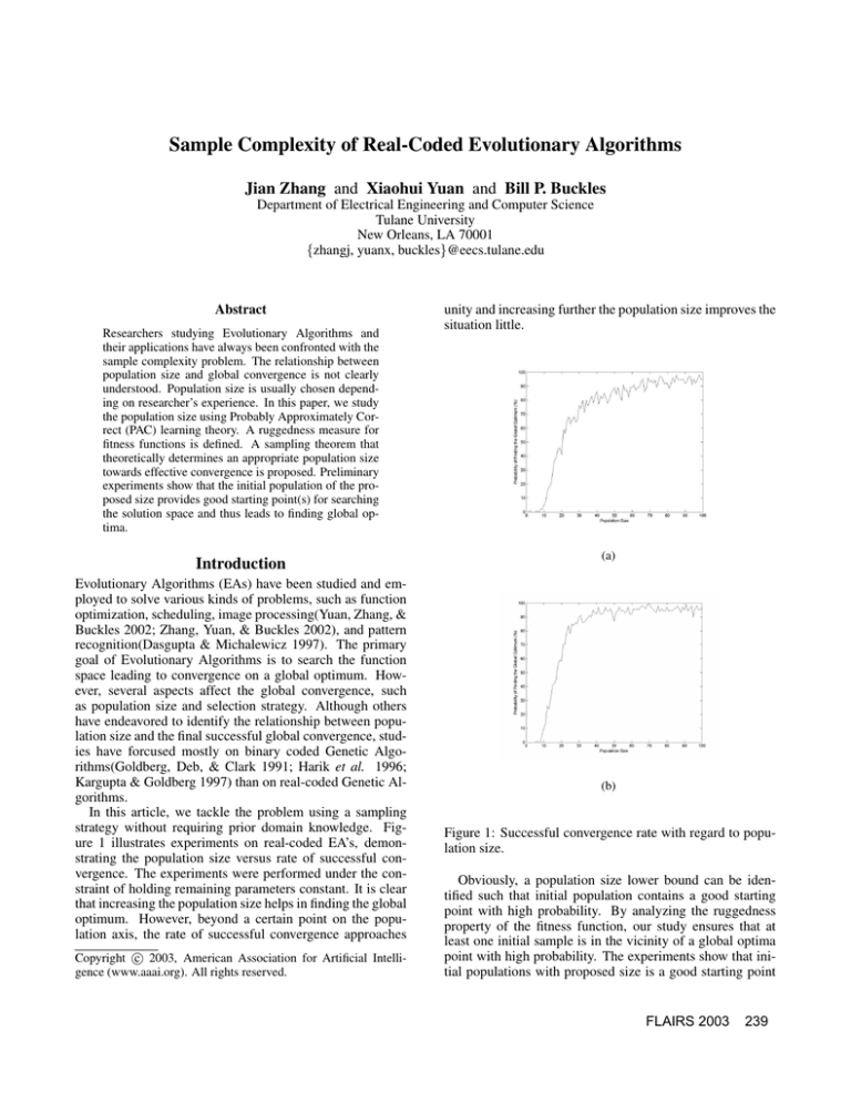
strategy without requiring prior domain knowledge. Figure 1 illustrates experiments on real-coded EA’s, demonstrating the population size versus rate of successful convergence. The experiments were performed under the constraint of holding remaining parameters constant. It is clear
that increasing the population size helps in finding the global
optimum. However, beyond a certain point on the population axis, the rate of successful convergence approaches
c 2003, American Association for Artificial IntelliCopyright gence (www.aaai.org). All rights reserved.
unity and increasing further the population size improves the
situation little.
(a)
(b)
Figure 1: Successful convergence rate with regard to population size.
Obviously, a population size lower bound can be identified such that initial population contains a good starting
point with high probability. By analyzing the ruggedness
property of the fitness function, our study ensures that at
least one initial sample is in the vicinity of a global optima
point with high probability. The experiments show that initial populations with proposed size is a good starting point
FLAIRS 2003
239
in the solution space and generally leads to convergence at
at an optimum. The rest of this paper is organized as follows. We first briefly review Probably Approximately Correct (PAC) learning theory and the prior work on determining PAC population sizes for a binary Genetic Algorithm.
Then a distance measure, i.e. granularity, in solution space
is defined and a theorem to determine the population size for
real-coded EAs is proposed. Last, experiments are presented
followed by discussion.
Background
The function optimization problem can be formalized as for
a given function f , which is defined on a real vector space
S, find x∗ ∈ S, such that ∀x ∈ S : f (x) > f ∗ , where
f ∗ = f (x∗ ) is the global minimum and x∗ is the global minimum point. With implicit parallelism, Evolutionary Algorithms quickly identify high performance regions within the
search space and converge to a global optimum represented
by (x∗ , f ∗ ).
Convergence Versus Population Size
The determination of population size is a compromise
choice that needs to be justified. Generally, a smallpopulation EA converges quickly, but finds global optima
with difficulty; a large-populatation EA has greater chance
of finding the solution in exchange for high computational
expense. The Schema Theorem(Holland 1975) and Walsh
transform have been used to analyze the convergence characteristics and population sizing of binary Genetic Algorithms(Goldberg & Rudnick 1991). Unfortunately, they neither prescribe how to sample the solution space or apply
to real-coded Evolutionary Algorithms. In fact, there is no
way to represent the infinite “building blocks” induced by
real-valued organisms. An initial attempt to bind the population size with the closeness to global optima points is
that of(Hernández-Aguirre, Buckles, & Martinez-Alcantara
2000). Using Probably Approximately Correct (PAC) learning theory, a population size for a binary GA is estimated so
that at least one of the initial individuals is d-bits away from
a global optimum, where 0 ≤ d ≤ l, l is the length of an
individual.
PAC Learning and Population Size for Binary GA
PAC learning is a theory of learning through examples. In
this section, we briefly review PAC learning and the prior
efforts on using PAC learning to study population size.
Let X be the set of all possible instances over which the
target function is defined and C refer to some subset of target
concepts that a learner might learn. The learner considers a
hypothesis space H when attempting to learn the target concept c. After observing a sequence of examples, a learner
must output a hypothesis h ∈ H that is a good approximation of c with high probability. In order to measure the
closeness of the output hypothesis h approximates the actual target concept c, the error of hypothesis h with respect
to c and a distribution D is defined as the probability that h
mismatches an instance drawn randomly according to D,
error(h) ≡ Pr (c(x) = h(x)),
240
FLAIRS 2003
where the probability Pr is over the distribution D. “High
probability” is indicated by the confidence parameter δ. The
number of training examples that is required by the learner
largely determines PAC-learnability. The minimum number
of training samples that is needed to attain PAC-learnability
is sample complexity(Mitchell 1997). The sample complexity m for finite hypothesis space is given as
1
1
(ln(|H|) + ln )
(1)
φ
δ
where φ is the bound on error(h), |H| is the size of hypothesis space H.
Hernandez et al. suggest sample complexity and population size are similar concepts.(Hernández-Aguirre, Buckles,
& Martinez-Alcantara 2000) By relating φ with d(h, h∗ ),
where h∗ is the target point (global optima point) and
d(h, h∗ ) is measured by Hamming distance between h and
h∗ , the PAC population size is determined for a binary GA.
m≥
Population Size of Evolutionary Algorithms
Ruggedness
Despite efforts that address the population size problem, its
relationship to fitness function has rarely been studied. Figure 2 illustrates two real value functions. Both functions
are defined over the same range of x and y (−50 ≤ x ≤
50, −50 ≤ y ≤ 50). However, they differ in their so called
ruggedness. It is obvious that the function illustrated in Figure 2(a) is more rugged than that of the function in Figure 2(b). A larger population size is required to effectively
optimize the function in Figure 2(a) (Zhang et al. 1999).
Intuitively, if the initial population of real-coded EAs is
large enough to include points that are in the neighborhood
of the global optimum, EAs have a great chance of locating the target point in subsequent generations. Although it
is generally true that a large population could guarantee the
closeness, how large is ‘large enough’ to ensure global convergence? To answer this question, a measurement inferring
closeness to optima points needs to be found.
Individuals in a population represent hypotheses in PAC
learning. In binary Genetic Algorithms, the hypothesis
space is finite and of size 2l , where l is the length of an
individual. The distance (i.e. error) between two individuals
(i.e. two hypotheses) is measured by Hamming distance. It
is proven that Hamming distance is an effective way to measure the closeness of optimization error in the binary case.
Whereas in real-coded EAs, the hypothesis space is tremendously large and it is infeasible to inherit the Hamming distance as the measure of the error. Therefore, we attempt to
infer the closeness measure from ruggedness of the function
and further induce the initial population size theorem.
Population Size of EAs
In this section, we define two important concepts, namely
granularity of fitness function and -cover. The population
size theorm as well as its proof are also described.
An approach to understanding function f is to decompose
it in terms of a pre-established function base, in order, it is
hoped, to reveal the important features of f .
solution space, then no point in that space is more than away from a member in -cover.
The following Theorem estimates the population size for
real-coded EAs such that given an initial population with the
proposed size, it forms an -cover of the solution space with
high probability and is essentially τ . That is, at least one
initial sample and a global optimum point are in the same
granule with high probability.
Theorem Given the fitness function f (x) with granularity
τ , where f (x) is defined on interval R, the PAC population
size m is bounded by m̃, that is, m ≥ m̃
1
1
1
m̃ = (ln
+ ln )
φ
φ
δ
(a)
(2)
where φ = τ /R and 1/φ defines the size of hypothesis
space, such that with confidence δ, 0 < δ < 1, the initial
population forms an -cover of R at probability greater than
1 − δ and = τ .
Proof Given function f (x), x ∈ R, let f¯(x) be the open
interval around a function value f (x). f ∗ represents the
open inverval around global optimum f (x∗ ), and is the target hypothesis in the solution space H. Given the granularity τ , φ = τ /R is the probability that for a sample x to be
drawn from H, d(x, x∗ ) ≤ τ .
(b)
√ 2 2
Figure 2: (a) f (x,√y) = e−0.02 x +y +cos x+sin y and (b)
2
2
f (x, y) = 50e−0.2 x +y + 5ecos(x/2)+sin(y/2) .
Definition: Granularity of Fitness Function A fitness function f (x) can be represented by the linear combination of a set of base functions B =
{b(g1 x), b(g2 x), . . . , b(gn x)}. The granularity of fitness
function f is defined as τ = 1/max(gi ), i = 1, 2, . . . , n,
where gi characterizes the frequency information of the base
function b.
Common choices of the function base are multiresolution
functions in both time domain and frequency domain, such
as sigmoid and wavelet functions.
The granularity property describes the local ruggedness
feature of the fitness function. That is, small granularity infers a more locally rugged function.
Here we adopt the definition of -cover provided by
Vidyasagar (Vidyasagar 1997).
Definition: -cover Let X be a set and function ξ :
X ×X → R+ be a pseudometric. Thus (X, ξ) forms a pseudometric space (metric space). Given S ⊆ X and > 0, a
set {α1 , α2 , . . . , αn } is an -cover of S if, for every x ∈ S,
there is a αi ∈ S such that ξ(x, αi ) ≤ .
Assume the initial population is drawn according to a uniform distribution. The population density increases with the
populaiton size. If initial population forms an -cover of the
τ
φ = p(d(x, x∗ ) ≤ τ ) = R
where p(.) is the probability function. Therefore
p(d(x, x∗ ) > τ ) = 1 − p(d(x, x∗ ) ≤ τ ) = 1 − φ
Assuming m samples are drawn independently from H,
∗
m
−φ
∩m
,
i=1 p(d(xi , x ) > τ ) = (1 − φ) . Since (1 − φ) ≤ e
(1 − φ)m < e−mφ
The size of hypothesis space |H| is the number of possible
intervals, i.e. number of f¯(x), with granularity τ in R,
|H| = R/τ = φ1 To bound the sampling error on |H| with δ, we have
|H|e−mφ ≤ δ
Therefore,
m ≥ φ1 (ln
φ1 + ln 1δ )
Because the population size is an integer, the population
size is bounded by m̃
2
m̃ = φ1 (ln
φ1 + ln 1δ )
Experiments
Based on the granularity definition and the population theorem, Algorithm 1 gives the PAC population size.
Algorithm 1 Estimating population size
Input error threshold δ
- determine the granularity τ of the given function f
- compute φ
- compute population size m using Eq. 2
FLAIRS 2003
241
Experiments have been performed on one dimensional
functions. However, it is easily extended to higher dimentional cases.
Table 1 lists the estimated PAC population size for functions illustrated in Figure 3. For demonstration purposes,
each function is repeated with population size from 1 to
100. At each population size 100 tests are performed. Based
on our proposed algorithm, a minimum population size that
satisfies the δ and -cover constraint is produced. The corresponding position in global convergence probability curve is
illustrated in Figure 4. The dashed line marks the PAC population size with error threshold δ = 0.1; the dash-dotted
line marks the PAC population size with δ = 0.05.
on a researcher’s experience. However, PAC learning provides a theory of learning from examples. Inspired by the
sample complexity concept in PAC learning theory, we study
the global convergence problem of EAs in terms of population size.
Taking advantage of the concept of granularity, we circumvent the difficulty of studying VC dimension of an infinite hypotheses space. A theoretical solution is developed
and experiments have been taken on one dimentational functions. Experiments verify that proposed PAC population
size minimizes the necessary number of initial individuals
to achieve the global convergence. Moreover, it can be easily extended to high dimentional functions.
References
Table 1: PAC population sizes.
Function
f1
f2
f3
Interval
[0,9]
[-10,10] [-5.12,5.12]
τ
1.2566 1.2566
1
φ
0.1369 0.0628
0.0977
Pop.Size (δ = 0.1)
33
81
49
Pop.Size (δ = 0.05)
38
92
56
From Figure 4 it can be seen that enlarging the population
size increases the probability of finding the global optimum.
However, after it reaches a certain point, the improvement
is no longer dramatic. The PAC population size is at the
threshold that gives high convergence rate and minimizes
the computational expense.
Table 2 lists the estimated PAC population size and the
corresponding convergence rate. The experiments demonstrate that the granularity of fitness functions effectively
measures closeness between individuals and that initial populations with the proposed size guarantee with high probability that the global optimum will be reached.
Table 2: PAC population size and probability of global convergence.
(δ = 0.1)
function
Interval
Pop. Size Prob. of Conv.
f1
[0, 9]
33
0.80
f2
[-10, 10]
81
0.72
f3
[-5.12, 5.12]
49
0.92
function
f1
f2
f3
(δ = 0.05)
Interval
Pop. Size
[0,9]
38
[-10, 10]
92
[-5.12, 5.12]
56
Prob. of Conv.
0.83
0.81
0.93
Conclusion
A PAC learning based population size estimation approach
for Evolutionary Algorithms is presented in this article. Population size for real-coded Evolutionary Algorithms is usually determined by ad hoc approaches and strongly depends
242
FLAIRS 2003
Dasgupta, D., and Michalewicz, Z., eds. 1997. Evolutionary Algorithms in Enigneering Applications. Berlin,
Germany: Springer.
Goldberg, D. E., and Rudnick, M. 1991. Genetic algorithms and the variance of fitness. Technical report no.
91001, Illinois genetic algorithms laboratory, University of
Illinois, Champaign-Urbana.
Goldberg, D. E.; Deb, K.; and Clark, J. H. 1991. Genetic
algorithms, noise, and the sizing of populaitons. Technical report no. 91010, Illinois genetic algorithms laboratory,
University of Illinois, Champaign-Urbana.
Harik, G.; Cantu-Paz, E.; Goldberg, D. E.; and Miller, B. L.
1996. Gambler’s ruin problem, genetic algorithms, and
the sizing of population. Technical report no. 96004, Illinois genetic algorithms laboratory, University of Illinois,
Champaign-Urbana.
Hernández-Aguirre, A.; Buckles, B. P.; and MartinezAlcantara, A. 2000. The PAC population size of a genetic
algorithm. In the 12th International Conference on Tools
with Artificial Intelligence, 199–202.
Holland, J. H. 1975. Adaptation in Natural and Artificial
Systems. Ann Arbor MI: University of Michigan Press.
Kargupta, H., and Goldberg, D. E. 1997. SEARCH, Blackbox Optimization, and Sample Complexity. San Francisco,
CA: Morgan Kaufmann. 291–324.
Mitchell, T. M. 1997. Machine Learning. McGraw-Hill.
Vidyasagar, M. 1997. A Theory of Learning and Generalization. Springer.
Yuan, X.; Zhang, J.; and Buckles, B. P. 2002. Feature
based approach for image correspondence estimation. In
Proceeding of the 2nd Int’l Conf. on Image and Graphics.
Zhang, J.; Yuan, X.; Zeng, Z.; Buckles, B. P.; Koutsougeras, C.; and Amer, S. 1999. Niching in an ES/EP
context. In Proceedings of Congress on Evolutionary Computation 1999.
Zhang, J.; Yuan, X.; and Buckles, B. P. 2002. An evolution strategies based approach to image registration. In
Proceeding of Genetic Evolutionary Computation Conference.
(a)
(a)
(b)
(b)
(c)
(c)
Figure 3: Functions (a) f1 (x) = x+10 sin 5x+7 cos 4x, x ∈
[0, 9]; (b) f2 (x) = x + 10 sin 5x + 7 cos 4x, x ∈ [−10, 10] ;
and (c) f3 (x) = 10 + x2 − 10 cos(2πx), x ∈ [−5.12, 5.12].
Figure 4: (a) convergence graph for function f1 . (b) convergence graph for function f2 . (c) convergence graph for
function f3 .
FLAIRS 2003
243