From: FLAIRS-00 Proceedings. Copyright © 2000, AAAI (www.aaai.org). All rights reserved.
Overriding the Experts: A Stacking Method For Combining Marginal Classifiers
Mark D. Happel and Peter Bock
Department of Computer Science
The George Washington University
Washington, DC 20052
mhappel@seas.gwu.edu & pbock@seas.gwu.edu
Abstract
The design of an optimal Bayesian classifier for
multiple features is dependent on the estimation of
multidimensional joint probability density functions
and therefore requires a design sample size that
increases exponentially with the number of
dimensions. A method was developed that combines
classifications from marginal density functions using
an additional classifier. Unlike voting methods, this
method can select a more appropriate class than the
ones selected by the marginal classifiers, thus
"overriding" their decisions. For two classes and two
features, this method always demonstrates a
probability of error no worse than the probability of
error of the best marginal classifier.
Introduction
Given a set of objects and their corresponding pattern
values, one of the fundamental problems of pattern
classification is to determine a mapping that can assign an
appropriate class label to each pattern in the pattern space.
In a Bayesian classifier, the classification decision is made
based on the a posteriori probabilities that the input is a
member of a pre-specified class given the input. For an
input pattern X, the a posteriori probability for class ωi,
p(ωi | X), can be calculated using Bayes’ rule, selecting the
class ωi for which p(X | ωi) P(ωi) > p(X | ωj) P(ωj) for all
i ≠ j. The Bayesian classifier is optimal in the sense that it
has the lowest possible probability of error for a given set
of probability density functions. If the probability of error
attained by a Bayesian classifier is unacceptably high for
the requirements of a given problem, a different feature
which exhibits better separation between the classes can be
sought. Alternatively, two or more features can be used
simultaneously to form multivariate joint probability
density functions.
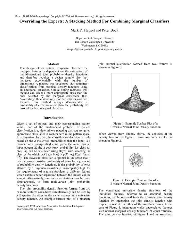
The joint probability density function formed from two
or more features considered simultaneously can be used by
a Bayesian classifier in the same manner as a univariate
density function. An example surface plot of a bivariate
Copyright © 1999, American Association for Artificial Intelligence
(www.aaai.org). All rights reserved.
joint normal distribution formed from two features is
shown in Figure 1.
M
Figure 1: Example Surface Plot of a
Bivariate Normal Joint Density Function
When viewed from directly above, the contours of the
density function in Figure 1 form concentric circles, as
shown in Figure 2.
M
Figure 2: Example Contour Plot of a
Bivariate Normal Joint Density Function
The constituent univariate density functions of the
individual features, referred to as marginal density
functions, can be obtained from the bivariate joint density
function by integrating the joint density function with
respect to one or the other of the coordinate axes. In the
case of Figure 1, integration yields uncorrelated features
with normal marginal density functions of equal variance.
The joint density function of Figure 1 and its associated
marginal densities are shown in Figure 3 below. Note that
the volume under the joint density curve, by definition, is
equal to one, as are the areas under the marginal density
curves.
M
Figure 3: Bivariate Normal Density and Associated
Marginal Densities
To better visualize the relationships between marginal
and bivariate density functions, a modified contour plot
such as the one shown in Figure 4 can be utilized. Here the
marginal densities are shown along their respective axes,
and a representative contour is plotted such that the
corresponding points of equal density are aligned. Note that
the contour line shown is only a single representative of the
actual contour (see Figure 2); a bivariate normal density
actually extends from -∞ to ∞ along both axes.
x2
p(x1 | ωi)
p(x1, x2 | ωi)
p(x1 | ωi)
x1
Figure 4: Modified Contour Plot for Figure 3
Bayesian classifiers provide optimal classification results
for a given pattern vector, provided that the classconditional density functions and a priori probabilities for
each class are known. Unfortunately, it is often the case
that these density functions are not known in advance and
must therefore be estimated from sample data. A wide
variety of parametric and nonparametric techniques for
estimating density functions exist and can be used for the
design of Bayesian classifiers (e.g., Bishop 1995; Fukunaga
1990; Scott 1992). The simplest nonparametric technique
for density estimation is the histogram, which records the
relative frequency with which samples fall within a given
range (bin width), thereby providing an estimate of the
average magnitude of the probability density function for
points falling within the bin.
There are several problems which tend to complicate the
use of histograms for the estimation of multivariate density
functions, including a dramatic increase in the number of
required histogram bins that can occur as the number of
dimensions is increased. Since the required number of bins
rises exponentially with an increasing number of
dimensions, it should be apparent that the resources
required to store and analyze such a histogram may quickly
exceed what is practical (Bishop 1995). This and other
related problems collectively contribute to what has
become known as "the curse of dimensionality" (Bellman
1961). The curse of dimensionality leads to an interesting
paradox: for situations in which the optimal Bayesian
classifier performance is insufficient for d dimensions, it
may not be possible in practice to attain better
classification performance using d+1 dimensions, even
though the theoretical Bayesian performance should
increase. From the preceding discussion, it is apparent that
a method for obtaining an improvement in the classification
performance for the d-dimensional Bayesian classifier
without requiring the estimation of d+1 dimensional
density functions would prove useful.
A promising line of research is based upon the creation
of a single "group" decision from the decisions of multiple
classifiers (Dietterich 1997). The performance of a
combination of classifiers has been found to be superior to
that of a single classifier in many situations. It is intuitively
appealing to imagine combining several, lower-dimensional
Bayesian classifiers in such a way as to provide a lower
error rate than any one of them alone can achieve, and
perhaps even to approach the error rate attainable with a
higher-dimensional classifier. Current strategies for
obtaining group decisions include dynamic classifier
selection (Woods, Kegelmeyer, and Bowyer 1997), voting
or weighted voting (Lam and Suen 1997), Bayesian
techniques (Bloch 1996; Xu, Krzyzak, and Suen 1992),
Dempster-Shafer evidence theory (Buede and Girardi
1997), and stacking methods (Dietterich 1997). Stacking
strategies, which use an additional classifier to combine the
results of the other classifiers, include the BehaviorKnowledge Space (BKS) approach, which stacked
handwriting recognition classifiers that were based on
different classification algorithms to obtain improved
performance (Huang and Suen 1995).
Solution Method
When two features x1 and x2 are available, they can be used
simultaneously by a bivariate classifier, whose block
diagram is shown in Figure 5. By using two features, the
bivariate classifier is often able to achieve a significantly
better classification performance than a comparable
univariate classifier that is relying on either of the same two
features. Unfortunately, the bivariate classifier will also
require a larger training sample size than the univariate
classifier to accurately estimate the class-conditional
probability density functions.
x2
M
M
B
x1
decision
Classifier
Classifier
ΨΨ1,2
x2
δ1,2
1,2
G
G
B
Figure 5: Bivariate Bayesian Classifier
M
The method proposed here is to use the marginal
decisions as features, thereby forming a new pattern vector.
An additional classifier, called a supervisory classifier, can
then be used to classify the pattern of marginal decisions
and generate a new classification decision. A block
diagram of this architecture is shown in Figure 6. Note that
this is essentially a stacking architecture, formed in this
case from multiple marginal classifiers and a single
supervisory classifier. The intention is to allow all of the
classifiers to be implemented from a single common
Bayesian building block. A version of this architecture has
been previously implemented and shown empirically to
improve recognition of printed characters (Happel and
Bock 1996).
x1
Classifier
Classifier
ΨΨ1
marginal
decision
δ1
B
x1
Figure 7: Probability Density Functions for
Two-Class Example
Using the architecture of Figure 6, feature x1 is classified
by marginal classifier Ψ1, while feature x2 is classified by
marginal classifier Ψ2. The marginal classifiers make a
Bayesian decision based only on the marginal density
functions for the single feature that they each receive. The
decision surface of each classifier is shown in Figure 8, and
the (one-dimensional) decision regions are shown along
each feature axis.
x2
M
1
1♦2
2
M
B
B
x2
decision
δ1♦2
M
Classifier
Classifier
ΨΨ1♦2
Classifier
Classifier
ΨΨ2
G
marginal
decision
δ2
In order to clarify the operation of this method, a detailed
example is presented in the next section.
B
G
Figure 6: Stacking Architecture
G
G
M
B
B
G
M
G
x1
An Example
Figure 8: Partitioning of the Joint Space
The example presented here involves three classes, labeled
"M", "B", and "G". Two features, x1 and x2, are used to
classify points in the feature space. The joint probability
density functions p(x1,x2 | M), p(x1,x2 | B), and p(x1,x2 | G)
are all normally-distributed, and the a priori probabilities
P(M), P(B), and P(G) are equal. The marginal density
functions p(x1 | M) and p(x2 | M) are normal, of equal
variance, and uncorrelated, as are p(x1 | B), p(x2 | B),
p(x1 | G) and p(x2 | G). The density functions are shown in a
modified contour plot in Figure 7.
The extension of the Bayesian decision surfaces from the x1
and x2 feature axes into the joint space divides the space
into η rectangular subdivisions called partitions. By
convention, partitions are labeled in the form
δ1δ2 according to the corresponding marginal decisions
δ1 and δ2 (i.e., the leftmost symbol will correspond to the
marginal decision made from feature x1). A partition
represents a portion of pattern space whose associated
patterns share common marginal decisions. The marginal
classifiers (Ψ1 and Ψ2 in Figure 6) receive features in
pattern space Π and transform them into marginal decisions
in partition space ρ on the basis of the class-conditional
pattern probability density functions p(χj | ωi). The
supervisory classifier (Ψ1♦2 in Figure 6) receives the
marginal decisions in partition space ρ and transforms them
to classification decisions in decision space ∆. To
accomplish this, the supervisory classifier requires the
class-conditional partition probabilities P(θk | ωi). The
supervisory classifier can use η bins to construct its
estimate of P(θk | ωi) for each class. If η is appreciably less
than the number of bins that would have been required to
estimate the joint probability density functions
p(x1,x2 | ωi), then the supervisory classifier will probably
require a smaller design sample size than would have been
required by a corresponding bivariate classifier using
p(x1,x2 | ωi).
The supervisory classifier will select the class ωi within
partition θk for which P(θk | ωi) is the largest. P(θk | ωi) is
equal to the volume of the class-conditional joint
probability density function p(x1,x2 | ωi) that is contained
within the boundaries of partition θk. Consequently, the
class selected by the supervisory classifier will be that class
whose probability density function p(x1,x2 | ωi) covers the
most volume within the partition in question.
This can be clearly seen for the current example in
Figure 9. Focusing on the upper right partition (GM), it is
readily apparent that the area under the class M bivariate
density function that falls within partition MM is much
larger than the area under the class B or G bivariate density
functions that also falls within partition MM. (It is
important to remember that the curves M and B of Figure
3-10 are merely representative contours of the bivariate
density functions, but the contours are useful for comparing
the respective volumes.) Consequently, a pattern that falls
within the partition is more likely to correspond to an
object from class M than one from classes B or G.
x2
BM
MM
Special attention should be paid to the center partition
(MB), which is shown in more detail in Figure 10. It is
readily apparent that the G class has the most volume under
its bivariate density function and therefore would be chosen
by the supervisory classifier. However, the marginal
classifiers chose classes M and B respectively. Thus, in this
case the supervisory classifier has overridden the advice of
the marginal classifiers with the result that a lower
probability of error is obtained. This override behavior is
not exhibited by more common classifier combination
techniques, such as majority voting, and is a key element in
the improved performance from this architecture.
M
MB
G
B
Figure 10: Decision Override in Partition MB
Similarly, the decision that would be made by the
supervisory classifier for the other partitions can be
predicted from Figure 9 and have been labeled in Figure 11
within the appropriate partitions.
x2
GM
MB
GB
B
G
G
B
G
G
G
G
M
G
B
BB
M
M
M
M
B
B
B
M
B
MG
M
BG
B
B
GG
G
G
M
Figure 9: Partition Labels Based on
Marginal Classifications
G
x1
B
M
Figure 11: Partition Classifications
G
x1
Note that the resultant decision surfaces, as shown in
Figure 12, are not identical to the decision surfaces from
either of the marginal classifiers, but have instead been
formed from a combination of them. Figure 12 also shows
the resultant probability of error, which is less than that of
either marginal classifier, as crosshatched volumes under
the respective density functions.
x2
Buede, D., and P. Girardi 1997. A Target Identification
Comparison of Bayesian and Dempster-Shafer Multisensor
Fusion. IEEE Transactions on Systems, Man, and
Cybernetics - Part A: Systems and Humans, 27(5):569577.
Dietterich, T. 1997. Machine Learning Research: Four
Current Directions. AI Magazine, Winter 1997:97-136.
M
B
Bloch, I. 1996. Information Combination Operators for
Data Fusion: A Comparative Review With Classification.
IEEE Transactions on Systems, Man and Cybernetics, Part
A, 26(1):52 -67.
M
Duda, R., and P. Hart 1973. Pattern Classification and
Scene Analysis. New York: John Wiley & Sons, Inc.
B
Fukunaga, K. 1990. Introduction to Statistical Pattern
Recognition (2nd ed.). Boston: Academic Press, Inc.
G
Happel, M. 1999. A Fusion Method for Combining
Marginal Classification Decisions using an OverrideCapable Classifier. Ph.D. dissertation proposal, Dept. of
Computer Science, The George Washington University.
G
B
M
G
x1
Figure 12: Resultant Probability of Error
Conclusions
The design of an optimal Bayesian classifier for multiple
features is dependent on the estimation of multidimensional
joint probability density functions and therefore requires a
design sample size that increases exponentially with the
number of dimensions. It has been shown above that it is
possible to combine the results of two marginal classifiers
and obtain a probability of error that is less than that of
either of the marginal classifiers. Further, it can be shown
that, for two classes with arbitrary bivariate density
functions, this method always demonstrates a probability of
error that is greater than or equal to the probability of error
of the optimal bivariate Bayesian classifier and less than or
equal to the probability of error of the marginal classifier
with the lowest probability of error (Happel 1999). Current
efforts are directed toward extending this result to an
arbitrary number of classes or dimensions, as well as
further characterizing the method's performance for
common parametric densities.
References
Bellman, R 1961. Adaptive Control Processes: A Guided
Tour. Princeton, NJ: Princeton University Press.
Bishop, C. 1995. Neural Networks for Pattern Recognition.
Oxford, UK: Oxford University Press.
Happel, M., and P. Bock 1996. The Classification of
Symbolic Concepts Using the ALISA Concept Module. In
Proceedings of the Ninth International Symposium on
Artificial Intelligence (ISAI-96), 170-179. Monterrey, N.L.,
Mexico: Instituto Technologico y de Estudious Superiores
de Monterrey (ITESM).
Huang, Y., and C. Suen 1995. A Method of Combining
Multiple Experts for the Recognition of Unconstrained
Handwritten Numerals. IEEE Transactions on Pattern
Analysis and Machine Intelligence 17(1):90-94.
Lam, L., and C. Suen 1997. Application of Majority Voting
to Pattern Recognition: An Analysis of Its Behavior and
Performance. IEEE Transactions on Systems, Man, and
Cybernetics - Part A: Systems and Humans 27(5):553-568.
Scott, D. 1992. Multivariate Density Estimation: Theory,
Practice, and Visualization. New York: John Wiley &
Sons.
Woods, K., W. Kegelmeyer Jr., and K. Bowyer 1997.
Combination of Multiple Classifiers using Local Accuracy
Estimates. IEEE Transactions on Pattern Analysis and
Machine Intelligence 19(4):405-410.
Xu, L., A. Krzyzak, and C. Suen 1992. Methods of
Combining Multiple Classifiers and Their Applications to
Handwriting Recognition. IEEE Transactions on Systems,
Man, and Cybernetics 22(3):418-435.