State-Variable (SV) Representations
1
Time-Domain Response of Second-Order Circuits:
In previous work circuits had been limited to one energy storage element, which
result in first order differential equations. Now, a second independent energy
storage element will be added to result in second order differential equations:
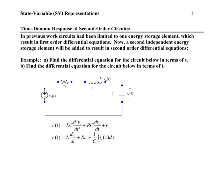
Example: a) Find the differential equation for the circuit below in terms of vc
b) Find the differential equation for the circuit below in terms of iL
iL(t)
R
L
C
vs(t)
dv
dv
v (t )  LC
 RC
v
dt
dt
di
1
v (t )  L
 Ri   i ( )d
dt
C
2
c
s
c
c
2
t
L
s
L

L
+
vc(t)
_
State-Variable (SV) Representations
2
Finding the Complete Solution for Second-Order Systems:
The method for determining the forced solution is the same for both first and
second order circuits. New aspects in solving a second order circuit involve new
forms of natural solutions that must be determined and two independent initial
conditions that must be found to resolve the unknown coefficients.
Finding the Natural Solution for second-order systems
1) Find characteristic equation of homogeneous equation (via Laplace Transform)
d x
dx
0
a
a x
dt
dt
2
2
1
2
d nx
Convert to polynomial by the following substitution: s  dt n
n
0  s 2  a1s  a2
2) Based on the roots of the characteristic equation, the natural solution will take on
one of three particular forms. Roots given by:
 a1  a12  4a2
s1, 2 
2
State-Variable (SV) Representations
3
a) If roots are real and distinct ( a  4a  0 ), natural solution becomes:
2
1
2
xn (t )  A1 exp( s1t )  A2 exp( s2t )
a1*exp(-t)+exp(-2t) for a1 =[-3:2]
3
2.5
2
response
1.5
a1=2
1
0.5
0
-0.5
-1
a1=-3
-1.5
-2
0
0.5
1
1.5
2
time
2.5
3
3.5
4
State-Variable (SV) Representations
4
b) If roots are real and repeated ( a  4a  0 ), natural solution becomes:
2
1
s1  s2
2
xn (t )  A1 exp( s1t )  A2t exp( s1t )
a1*exp(-t)+t*exp(-t) for a1 =[-3:2]
2
a1=2
1.5
1
response
0.5
0
-0.5
-1
a1=-3
-1.5
-2
-2.5
-3
0
0.5
1
1.5
2
time
2.5
3
3.5
4
State-Variable (SV) Representations
5
c) If roots are complex ( a  4a  0 ), natural solution becomes:
2
S1, 2    j
or
1
2
x (t )  exp( t ) c cos( t )  c sin( t )
x (t )  A exp( t ) cos(  t   )
n
1
2
n
exp(-t).*(cos(6*pi*t)+2*sin(6*pi*t))
2.5
2
1.5
response
1
0.5
0
-0.5
-1
-1.5
-2
0
0.5
1
1.5
2
time
2.5
3
3.5
4
State-Variable (SV) Representations
6
Find the step response for vc and iL for the circuit below:
iL(t)
R
vs(t)
L
C
+
vc(t)
_
when
a) R=16, L=2H, C=1/24 F
b) R=10, L=1/4H, C=1/100 F
c) R=2, L=1/3H, C=1/6 F
Show:
3
1
 1

a) v (t )   1  exp( 6t )  exp( 2t ) u(t ) iL (t )  3 exp( 2t )  3 exp( 6t ) u (t )
 2

2
24
b) v (t )  1  exp( 20t )  20t exp( 20t )u(t ) iL (t )  4t exp( 20t ) u(t )
c) v (t )  1  exp( 3t )cos(3t )  sin(3t )u(t ) iL (t )  exp( 3t ) sin( 3t )u(t )
c
c
c
State-Variable (SV) Representations
%
%
This script will plot the step response of voltage and current in
the 3 cases of the series RLC circuit example in lecture notes
t = [0:.01:2.5];
% Create time axis (at least 5 times the largest
% time constant in length
% Compute Capacitor voltage expressions
vca = (1+0.5*exp(-6*t)-1.5*exp(-2*t));
vcb = (1-exp(-20*t)-20*t.*exp(-20*t));
vcc =(1-exp(-3*t).*(cos(3*t)+sin(3*t)));
% Compute Inductor current expression
ila = (1/24)*(3*exp(-2*t)-3*exp(-6*t));
ilb = 4*t.*exp(-20*t);
ilc = exp(-3*t).*sin(3*t);
% Plot and label voltages and currents
figure(1)
plot(t,vca)
xlabel('seconds')
ylabel('volts')
title('Part a, Capacitor Voltage')
figure(2)
plot(t,ila)
xlabel('seconds')
ylabel('amps')
7
State-Variable (SV) Representations
8
title('Part a, Inductor Current')
............
continue similar statement for parts b and c
Part a, Inductor Current
Part b, Inductor Current
0.05
0.045
Part c, Inductor Current
0.08
0.35
0.07
0.3
0.06
0.25
0.05
0.2
0.04
amps
amps
0.03
0.025
0.02
amps
0.035
0.04
0.15
0.03
0.1
0.02
0.05
0.01
0
0.015
0.01
0.005
0
0
0.5
1
1.5
2
0
2.5
0
0.5
1
seconds
1.5
2
2.5
-0.05
0
0.5
1
seconds
Part a, Capacitor Voltage
Part b, Capacitor Voltage
1
1
0.9
0.9
0.8
0.8
0.7
0.7
0.6
0.6
1.5
2
2.5
2
2.5
seconds
Part c, Capacitor Voltage
1.4
0.5
1
0.8
volts
volts
volts
1.2
0.5
0.4
0.4
0.3
0.3
0.2
0.2
0.1
0.1
0.6
0.4
0.2
0
0
0.5
1
1.5
seconds
2
2.5
0
0
0.5
1
1.5
seconds
2
2.5
0
0
0.5
1
1.5
seconds
State-Variable (SV) Representations
9
Matrix Method for Describing Differential Equations:
A more systematic way to find the differential equations is to express them directly
in terms the independent voltages and currents in the system. Consider the circuit
below as an example:
iL(t)
R
vs(t)
L
C
+
vc(t)
_
A general approach:
1. Identify the independent voltages and/or currents in the circuit. These are values
that you need initial conditions for in order to solve for the unique complete
solution (i.e. capacitor voltages and inductor currents).
2. Find an equation for each independent value that relates its first derivative to
zero-order derivatives of the other independent values and sources.
3. Set up a system of first order differential equations in a matrix form.
4. Express the particular output value in terms of a linear combination of the
independent values. Use matrix notation.
State-Variable (SV) Representations
10
Example:
For the circuit below find the differential equations and output equation in matrix
form, where the output is v0:
1H
is
1mF
1 k
Show:
 i   1000 1   i
v    1000  1 v

  
L
L
C
C
  0 
  1000i
 

s
+
v0
-
i
v  1000 0 
v
L
0
C
1k

   0i

s
State-Variable (SV) Representations
11
Example:
For the circuit below find the differential equations and output equation in matrix
form, where the output is v0:
is
1
F
3
9
vs
1
F
2
Show:
v   7 / 18 1 / 6  v  2 2 / 9  i 
v    1 / 4
 v   0

1
/
4
0  v 
  
  
C1
C2
C1
C2
s
s
+
v0
-
12
v 
i 
v  1  1     0 0  
v 
v 
C1
s
C2
s
0