Strategic Sales Management in an Autonomous Trading Agent for TAC SCM
Wolfgang Ketter, Eric Sodomka, Amrudin Agovic, John Collins, and Maria Gini
Department of Computer Science and Engineering, University of Minnesota, Minneapolis, MN 55455, USA
{ketter,sodomka,aagovic,jcollins,gini}@cs.umn.edu
Introduction
Regime Identification and Prediction
To operate successfully in a competitive trading environment such as the Trading Agent Competition for Supply
Chain Management (Collins et al. 2004) (TAC SCM), an
agent has to allocate resources and set prices in a way that
maximizes its expected profit. This requires the ability to
detect changing market conditions and act accordingly.
In TAC SCM six agents buy parts, assemble personal
computers, and sell them in daily auctions to customers.
Sales decisions in our agent, MinneTAC, are driven by
three different models: an automated characterization and
prediction of market conditions, which we call economic
regimes (Ketter 2005), a linear program that optimizes daily
sales quotas, and a model of order acceptance probability.
While economic regime models are commonly used at the
macro economic level (Osborn & Sensier 2002), such predictions are rarely done for a micro economic environment.
We focus on the sales decisions the agent has to make,
where predicting prices and customer demand play an essential role. The strategies we present have been inspired,
among others, by the work of Kephart et al. (Kephart, Hanson, & Greenwald 2000).
MinneTAC makes sales decisions in two steps. The first
step is a strategic decision, where resources are allocated
over a planning horizon in a way that maximizes expected
profit over the horizon. The second step is a tactical decision, which determines the offer prices that are expected to
sell the quantities determined by the strategic decision, given
the current demand and the pricing model.
Off-line Regime Characterization. We characterize market regimes by analyzing off-line data from previous games.
The agent then uses these results along with real-time observable information to identify regimes during the game,
forecast regime transitions, and adapt its procurement, production, and pricing strategies accordingly. For our experiments, we used training data from a set of 24 games played
during the semi-finals and finals of TAC SCM 2005.
Agents can build and sell many different types of computers. Each computer type has a nominal price, which is the
sum of the nominal cost of the parts needed to build it. We
normalize the prices across the different computer types. We
call np the normalized price.
We define regimes with a Gaussian mixture model
(GMM). We use a GMM with fixed means, µi , and fixed
variances, σi , since we want the same set of Gaussians to
work for all games. We use the Expectation-Maximization
(EM) Algorithm to demarginalize the GMM and determine the prior probability, P (ci ), of the Gaussian components. The density of the normalized price can be written
PN
as p(np) = i=1 p(np|ci ) P (ci ), where p(np|ci ) is the ith Gaussian from the GMM. For our experiments we chose
N = 16, because we found experimentally that this works
well for price trend predictions.
Using Bayes’ rule we determine the posterior probability
P (c|np). We then define the N-dimensional vector
~η (np) = [P (c1 |np), P (c2 |np), . . . , P (cN |np)]
whose components are the posterior probabilities from the
GMM, and for each normalized price npj we compute
~η (npj ) which is ~η evaluated at the npj price. We cluster
these collections of vectors using the k-means algorithm.
The center of each cluster is a probability vector that corresponds to regime r = Rk for k = 1, · · · , M , where M is
the number of regimes.
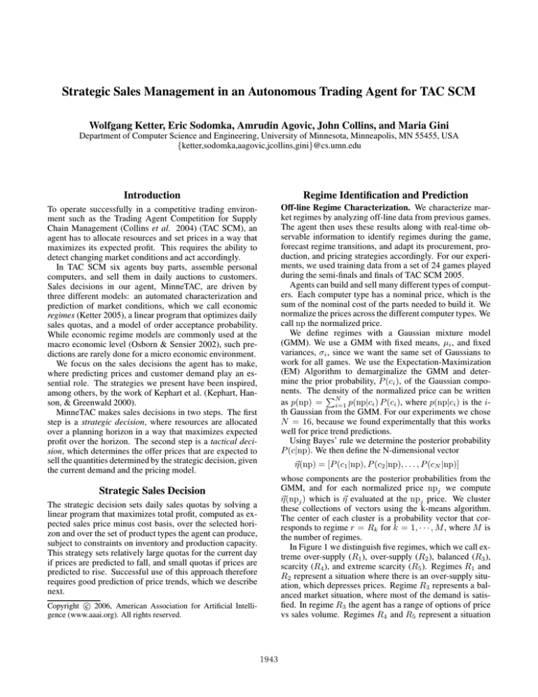
In Figure 1 we distinguish five regimes, which we call extreme over-supply (R1 ), over-supply (R2 ), balanced (R3 ),
scarcity (R4 ), and extreme scarcity (R5 ). Regimes R1 and
R2 represent a situation where there is an over-supply situation, which depresses prices. Regime R3 represents a balanced market situation, where most of the demand is satisfied. In regime R3 the agent has a range of options of price
vs sales volume. Regimes R4 and R5 represent a situation
Strategic Sales Decision
The strategic decision sets daily sales quotas by solving a
linear program that maximizes total profit, computed as expected sales price minus cost basis, over the selected horizon and over the set of product types the agent can produce,
subject to constraints on inventory and production capacity.
This strategy sets relatively large quotas for the current day
if prices are predicted to fall, and small quotas if prices are
predicted to rise. Successful use of this approach therefore
requires good prediction of price trends, which we describe
next.
c 2006, American Association for Artificial IntelliCopyright gence (www.aaai.org). All rights reserved.
1943
0
1
0.8
0.7
R1
R2
R3
R4
R5
−0.02
−0.04
−0.06
0.6
Price Trend
k
Regime Probability P(R |np)
0.9
0.5
0.4
−0.08
−0.1
−0.12
−0.14
0.3
−0.16
0.2
−0.18
0.1
−0.2
0
0
0.25
0.5
0.75
Normalized Price
1
M 5%
M 10%
M 50%
Real Mean
12
1.25
14
16
18
20
22
Day
24
26
28
30
Figure 2: Predicted price trend from day 10 to day 30. The
solid curve is the real mean price trend and the dashed and
dotted curves are predicted prices trends based on the 5%,
10% and 50% percentiles of the predicted price density.
Figure 1: Regime probabilities over normalized price.
where there is scarcity of products, which increases prices.
In this case the agent should price close to the customer reserve price – the maximum price a customer is willing to
pay.
We marginalize the product of p(np|ci ) and P (ci |Rk )
over all Gaussians ci to obtain P (np|Rk ). The probability of regime Rk dependent on the normalized price np can
be computed using Bayes rule as:
Tactical Sales Decision
Given the daily sales quotas, price trend predictions, and the
current demand dg , the final decision is to set the highest
possible offer price op g for each product g at which g’s sales
are expected to reach its desired quota qg . We maintain a
current pricing model that approximates the probability that
customers will accept an offer. This is a simple linear approximation giving the expected median price mg (derived
from np) and slope sg of the acceptance probability function. Using this model, the offer price op g for each product
is
1 qg
1
op g =
−
+ mg .
sg dg
2
P (np|Rk ) P (Rk )
P (Rk |np) = PM
∀k = 1, · · · , M.
k=1 P (np|Rk ) P (Rk )
where M is the number of regimes, which in our case is 5.
The prior probabilities P (Rk ) of the different regimes are
determined by a counting process over multiple games. Figure 1 depicts the regime probabilities for a sample market.
Online Regime Identification. During the game, the
agent estimates the current regime every day by calculating the mid-range normalized price npday for the day and
by selecting the regime with the highest probability, i.e.
argmax1≤k≤M P~ (Rk |npday ). The mid-range price is computed from the daily report of the minimum and maximum
prices of the computers sold the day before.
Online Regime Prediction. Since regimes are correlated
with prices, predicting regime changes can help predicting
price changes. We model regime prediction as a Markov
process and construct a transition matrix off-line by a counting process over past games. This matrix represents the
posterior probability of transitioning in day t + 1 to a
regime given the current regime in day t . The prediction is based on two distinct operations: (1) a correction
(recursive Bayesian update) of the posterior probabilities
P~ (rt−1 |{npt0 , . . . , npt−1 }) for the regimes based on the
history of measurements of the mid-range normalized price
np from the day of the last regime change, t0 , to the previous
day, t − 1, and (2) a prediction of the regime posterior probabilities for the current day, t, P~ (rt |{npt0 , . . . , npt−1 }).
Price Density and Trend Prediction. The agent predicts
the price density using the predicted regime distribution and
the learned GMM for every day over the planning horizon
n using a range of values for np. To predict price trends
we track the 5%, 10%, and 50% percentiles of the predicted
price density. Figure 2 shows price trends for a sample game
from day 10 until day 30. These predicted price trends are
then used to compute optimal sales quotas.
Offer prices are slightly randomized, and actual sales performance is used to update the model.
Conclusions and Future Work
We have described an approach to sales decision-making
that uses economic regimes, resource allocation, and prediction of order probabilities. The approach presented is focuses on sales decisions, but price trends can also be used
for decision making in procurement and production.
References
Collins, J.; Arunachalam, R.; Sadeh, N.; Ericsson, J.;
Finne, N.; and Janson, S. 2004. The Supply Chain Management Game for the 2005 Trading Agent Competition. Technical Report CMU-ISRI-04-139, Carnegie Mellon University, Pittsburgh, PA.
Kephart, J. O.; Hanson, J. E.; and Greenwald, A. R. 2000.
Dynamic pricing by software agents. Computer Networks
32(6):731–752.
Ketter, W. 2005. Dynamic Regime Identification and Prediction Based on Observed Behavior in Electronic Marketplaces. In Proc. of the Twentieth National Conference on
Artificial Intelligence, 1646–1647.
Osborn, D. R., and Sensier, M. 2002. The prediction of
business cycle phases: financial variables and international
linkages. National Institute Econ. Rev. 182(1):96–105.
1944