Hidden Naive Bayes
Harry Zhang
Faculty of Computer Science
University of New Brunswick, Canada
E3B 5A3, hzhang@unb.ca
Liangxiao Jiang
Faculty of of Computer Science
China University of Geosciences
Wuhan, China 430074
Abstract
Jiang Su
Faculty of Computer Science
University of New Brunswick, Canada
E3B 5A3, k4km1@unb.ca
use c to represent the value that C takes and c(E) to denote the class of E. The Bayesian classifier represented by a
Bayesian network is defined in Equation 1.
The conditional independence assumption of naive
Bayes essentially ignores attribute dependencies and is
often violated. On the other hand, although a Bayesian
network can represent arbitrary attribute dependencies,
learning an optimal Bayesian network from data is intractable. The main reason is that learning the optimal structure of a Bayesian network is extremely time
consuming. Thus, a Bayesian model without structure
learning is desirable. In this paper, we propose a novel
model, called hidden naive Bayes (HNB). In an HNB,
a hidden parent is created for each attribute which
combines the influences from all other attributes. We
present an approach to creating hidden parents using
the average of weighted one-dependence estimators.
HNB inherits the structural simplicity of naive Bayes
and can be easily learned without structure learning.
We propose an algorithm for learning HNB based on
conditional mutual information. We experimentally test
HNB in terms of classification accuracy, using the 36
UCI data sets recommended by Weka (Witten & Frank
2000), and compare it to naive Bayes (Langley, Iba, &
Thomas 1992), C4.5 (Quinlan 1993), SBC (Langley &
Sage 1994), NBTree (Kohavi 1996), CL-TAN (Friedman, Geiger, & Goldszmidt 1997), and AODE (Webb,
Boughton, & Wang 2005). The experimental results
show that HNB outperforms naive Bayes, C4.5, SBC,
NBTree, and CL-TAN, and is competitive with AODE.
(1)
c(E) = arg max P (c)P (a1 , a2 , · · · , an |c).
c∈C
Assume that all attributes are independent given the class;
that is,
P (E|c) = P (a1 , a2 , · · · , an |c) =
n
Y
P (ai |c).
(2)
i=1
The resulting classifier is called a naive Bayesian classifier,
or simply naive Bayes:
c(E) = arg max P (c)
c∈C
n
Y
(3)
P (ai |c).
i=1
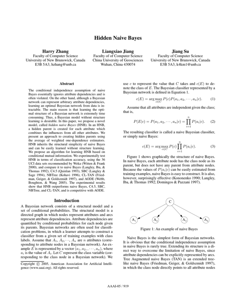
Figure 1 shows graphically the structure of naive Bayes.
In naive Bayes, each attribute node has the class node as its
parent, but does not have any parent from attribute nodes.
Because the values of P (ai |c) can be easily estimated from
training examples, naive Bayes is easy to construct. It is also,
however, surprisingly effective (Kononenko 1990; Langley,
Iba, & Thomas 1992; Domingos & Pazzani 1997).
Introduction
C
A Bayesian network consists of a structural model and a
set of conditional probabilities. The structural model is a
directed graph in which nodes represent attributes and arcs
represent attribute dependencies. Attribute dependencies are
quantified by conditional probabilities for each node given
its parents. Bayesian networks are often used for classification problems, in which a learner attempts to construct a
classifier from a given set of training examples with class
labels. Assume that A1 , A2 ,· · ·, An are n attributes (corresponding to attribute nodes in a Bayesian network). An example E is represented by a vector (a1 , a2 , , · · · , an ), where
ai is the value of Ai . Let C represent the class variable (corresponding to the class node in a Bayesian network). We
c 2005, American Association for Artificial IntelliCopyright gence (www.aaai.org). All rights reserved.
A1
A2
A3
A4
Figure 1: An example of naive Bayes
Naive Bayes is the simplest form of Bayesian networks.
It is obvious that the conditional independence assumption
in naive Bayes is rarely true. Extending its structure is a direct way to overcome the limitation of naive Bayes, since
attribute dependencies can be explicitly represented by arcs.
Tree Augmented naive Bayes (TAN) is an extended treelike naive Bayes (Friedman, Geiger, & Goldszmidt 1997),
in which the class node directly points to all attribute nodes
AAAI-05 / 919
and an attribute node can have only one parent from another
attribute node. Figure 2 shows an example of TAN. TAN is
a specific case of general Augmented naive Bayesian networks, or simply Augmented naive Bayes (ANB), in which
the class node also directly points to all attribute nodes, but
there is no limitation on the arcs among attribute nodes (except that they do not form any directed cycle).
C
A1
A2
A3
A4
As discussed in the previous section, ANB is an example of the second approach. Learning restricted ANB, such
as TAN, is a reasonable trade-off between model optimality and computational complexity. In fact, Friedman et al.
(1997) show that the result of searching for an optimal
Bayesian network may not be better than the result of just
searching for an optimal TAN. They propose a TAN learning
algorithm based on conditional mutual information between
two attributes given the class variable, called CL-TAN in this
paper. CL-TAN is an extension of the ChowLiu algorithm
(Chow & Liu 1968). The conditional mutual information is
defined as
IP (X; Y |Z) =
X
x,y,z
Figure 2: An example of TAN
Learning an optimal ANB is equivalent to learning an optimal Bayesian network, which has been proved to be NPhard (Chickering 1996). In fact, the most time consuming
step in learning a Bayesian network is learning the structure (structure learning). In practice, imposing restrictions
on the structures of Bayesian networks, such as TAN, leads
to acceptable computational complexity and a considerable
improvement over naive Bayes. One main issue in learning
TAN is that only one attribute parent is allowed for each attribute, ignoring the influences from other attributes. In addition, in a TAN learning algorithm, structure learning is also
unavoidable.
Certainly, a model that avoids structure learning, and is
still able to represent attribute dependencies to some extent,
is desirable. In this paper, we present a new model hidden
naive Bayes (HNB). HNB creates a hidden parent for each
attribute, which represents the influences from all other attributes. Our experimental results show that HNB demonstrates remarkable accuracy compared to other state-of-theart algorithms.
The rest of the paper is organized as follows. We first introduce the related work. Then we present our new model
hidden naive Bayes, followed by the description of our experimental setup and results in detail. We make a conclusion
and outline the main directions for future research.
Related Work
Numerous techniques have been proposed to improve or extend naive Bayes, mainly in two approaches: selecting attribute subsets in which attributes are conditionally independent, and extending the structure of naive Bayes to represent
attribute dependencies.
The idea of selecting a subset of attributes or forming new
attributes is to convert the data to a new form that satisfies the conditional independence assumption. Of the proposed techniques, selective naive Bayes (SBC) by Langley
and Sage (1994) demonstrates a remarkable improvement
over naive Bayes. SBC uses forward selection to find a good
subset of attributes, and then uses this subset to construct a
naive Bayes.
P (x, y, z)log
P (x, y|z)
,
P (x|z)P (y|z)
(4)
where x, y, and z are the values of variables X, Y , and
Z respectively. In CL-TAN, IP (Ai ; Aj |C) between each
pair of attributes is computed, and a complete undirected
weighted graph is built, in which nodes are attributes A1 ,
· · ·, An , and the weight of an edge connecting Ai to Aj is
set to IP (Ai ; Aj |C). Then, a maximum weighted spanning
tree is constructed. Finally, the undirected tree is converted
to directed, and a node labeled by C that points to all attribute nodes is added. Keogh and Pazzani (1999) propose
a cross-validation-based TAN learning algorithm SuperParent, and show that the SuperParent algorithm outperforms
the CL-TAN learning algorithm in classification accuracy.
However, its training time complexity is also significantly
higher than that of CL-TAN.
Kohavi (1996) presents a model NBTree to combine a decision tree with naive Bayes. In an NBTree, a local naive
Bayes is deployed on each leaf of a traditional decision tree,
and an example is classified using the local naive Bayes
on the leaf into which it falls. The experiments show that
NBTree outperforms naive Bayes significantly in accuracy.
The most recent work on improving naive Bayes is AODE
(averaged one-dependence estimators) (Webb, Boughton, &
Wang 2005). In AODE, an ensemble of one-dependence
classifiers are learned and the prediction is produced by
aggregating the predictions of all qualified classifiers. The
notion of x-dependence is introduced by Sahami (Sahami
1996). An x-dependence estimator means that the probability of an attribute is conditioned by the class variable and
at most x other attributes, which corresponds to an ANB
with at most x attribute parents. In AODE, a one-dependence
classifier is built for each attribute, in which the attribute is
set to be the parent of all other attributes. Their experimental results show that AODE performs surprisingly well compared to other classification algorithms. For example, AODE
outperforms the SuperParent algorithm significantly.
Some other, more sophisticated, naive Bayes-based learning algorithms with high time complexity have also been
proposed. Zhang (2004) proposes a model, hierarchical
naive Bayes, in which hidden variables are introduced to alleviate the conditional independence assumption. A hierarchical naive Bayes is a tree-like Bayesian network in which
internal nodes are hidden variables, and leaf nodes are attributes. Learning hierarchical naive Bayes has a high com-
AAAI-05 / 920
putational complexity. Zheng and Webb (2000) propose an
approach of lazy learning, the lazy Bayesian rule (LBR). The
time complexity for learning LBR is also quite high.
The classifier corresponding to an HNB on an example
E = (a1 , · · · , an ) is defined as follows.
c(E) = arg max P (c)
Hidden Naive Bayes
c∈C
As discussed in previous sections, naive Bayes ignores
attribute dependencies. On the other hand, although a
Bayesian network can represent arbitrary attribute dependencies, it is intractable to learn it from data (Chickering
1996). Thus, learning restricted structures, such as TAN,
is more practical. However, only one parent is allowed for
each attribute in TAN, even though several attributes might
have the similar influence on it. Our motivation is to develop
a new model that can avoid the intractable computational
complexity for learning an optimal Bayesian network and
still take the influences from all attributes into account. Our
idea is to create a hidden parent for each attribute, which
combines the influences from all other attributes. This model
is called hidden naive Bayes (HNB).
C
A1
Ahp
1
A2
A3
Ahp
Ahp
2
......
......
3
An
Ahp
n
Figure 3: The structure of HNB
Figure 3 gives the structure of an HNB. In Figure 3, C is
the class node, and is also the parent of all attribute nodes.
Each attribute Ai has a hidden parent Ahpi , i = 1, 2, · · · , n,
represented by a dashed circle. The arc from the hidden parent Ahpi to Ai is also represented by a dashed directed line,
to distinguish it from regular arcs.
The joint distribution represented by an HNB is defined
as follows.
n
Y
P (A1 , · · · , An , C) = P (C)
P (Ai |Ahpi , C), (5)
i=1
where
P (Ai |Ahpi , C) =
n
X
j=1,j6=i
Wij ∗ P (Ai |Aj , C),
(6)
Pn
and j=1,j6=i Wij = 1. The hidden parent Ahpi for Ai
is essentially a mixture of the weighted influences from all
other attributes.
n
Y
P (ai |ahpi , c).
(7)
i=1
In an HNB, attribute dependencies are represented by
hidden parents of attributes. The way of defining hidden
parents determines the capability of representing attribute
dependencies. In Equation 6, one-dependence estimators
P (Ai |Aj , C) are used to define hidden parents. Recall that
at most one attribute parent is allowed for each attribute in
TAN, and the influences from other attributes have to be ignored. In an HNB, on the other hand, the influences from
all other attributes can be represented and a weight is used
to represent the importance of an attribute. Thus, intuitively,
HNB is a more accurate and expressive model than TAN
with respect to representing attribute dependencies.
If we have an order of attributes: A1 , · · ·, An ,
P (Ai |Ahpi , C) can be thought of as an approximation of
P (Ai |A1 , · · · , Ai−1 ). In Equation 6, the approximation is
based on one-dependence estimators. However, in principle,
arbitrary x-dependence estimators can be used to define hidden parents. If x = n − 1, any Bayesian network is representable by an HNB. Thus, theoretically, an HNB is equivalent to a Bayesian network in terms of expressive power. In
practice, however, we would prefer a simple way to define
hidden parents in order to make the learning process simple
and efficient.
From Equation 5 and 6, we can see that the approach to
determining the weights Wij , i, j = 1, · · · , n and i 6= j,
is crucial for learning an HNB. There are two general approaches to doing it: performing a cross-validation based
search, or directly computing the estimated values from data.
We adopt the latter, and use the conditional mutual information between two attributes Ai and Aj as the weight of
P (Ai |Aj , C). More precisely, in our implementation, Wij
is defined in Equation 8.
IP (Ai ; Aj |C)
,
j=1,j6=i IP (Ai ; Aj |C)
Wij = Pn
(8)
where IP (Ai ; Aj |C) is the conditional mutual information defined in Equation 4.
Learning an HNB is quite simple and mainly about estimating the parameters in the HNB from the training data.
The learning algorithm for HNB is depicted as follows.
Algorithm HNB(D)
Input: a set D of training examples
Output: an hidden naive Bayes for D
for each value c of C
Compute P (c) from D.
for each pair of attributes Ai and Aj
for each assignment ai , aj , and c to Ai , Aj , and C
Compute P (ai , aj |c) from D
for each pair of attributes Ai and Aj
Compute IP (Ai , Aj |C)
for each attribute AiP
n
Compute Wi = j=1,j6=i IP (Ai ; Aj |C)
AAAI-05 / 921
for each attribute Aj and j 6= i
I (Ai ,Aj |C)
Compute Wij = P W
i
Table 1: Description of the data sets used in the experiments.
From the algorithm above, we know that the training
process of HNB is similar to CL-TAN, except no structure
learning. A three-dimensional table of probability estimates
for each attribute-value, conditioned by each other attributevalue and each class is generated. To create the hidden parent
of an attribute, HNB needs to compute the conditional mutual information IP (Ai ; Aj |C) for each pair of attributes.
The time complexity for computing weights using Equation
8 is O(n2 ). Thus, the training time complexity of HNB is
O(tn2 +kn2 v 2 ), where t is the number of training examples,
n is the number of attributes, k is the number of classes, and
v is the average number of values for an attribute. At classification time, given an example, Equation 7 is used, and it
takes O(kn2 ).
Compared to CL-TAN, which has a training time complexity of O(tn2 + kn2 v 2 + n2 logn) and classification time
complexity of O(kn), HNB does not have structure learning
with the time complexity of O(n2 logn) in CL-TAN. Thus,
the training time complexity of HNB is lower than that of
CL-TAN.
Compared to AODE, which has a training time complexity of O(tn2 ) and classification time complexity of O(kn2 ),
HNB needs more training time and same classification time.
HNB, however, has an explicit semantics. Roughly speaking, a hidden parent for an attribute can be seen as aggregating the influences from all other attributes that with higher
influences are assigned higher weights. Such an explicit semantics makes HNB understandable. In real-world applications, the comprehensibility of a model is important for
decision making. Actually, the weights in HNB can be assigned by human experts, which allows an effective interaction between human experts and the learning program. In
addition, we should notice that AODE is an ensemble learning method, in which a collection of models is built and their
predictions are combined, whereas only a single model is
learned in HNB.
Experiments and Results
We ran our experiments on all the 36 data sets recommended
by Weka (Witten & Frank 2000), which are described in Table 1. All these data sets are from the UCI repository (Blake
& Merz 2000). We downloaded these data sets in the format
of arff from the main web of Weka.
In the preprocessing stages of data sets, we used the filter of ReplaceMissingValues in Weka to replace the missing
values of attributes. Numeric attributes were discretized by
the filter of Discretize in Weka using unsupervised ten-bin
discretization. Thus, all attributes were treated as nominal.
Moreover, it is well-known that, if the number of values of
an attribute is almost equal to the number of examples in a
data set, this attribute does not contribute any information to
classification. So we used the filter of Remove in Weka to
delete this type of attribute.
In our experiments, we used the Laplace estimation to
avoid the zero-frequency problem. More precisely, we esti-
data set
anneal
anneal.ORIG
audiology
autos
balance-scale
breast-cancer
breast-w
colic
colic.ORIG
credit-a
credit-g
diabetes
Glass
heart-c
heart-h
heart-statlog
hepatitis
hypothyroid
ionosphere
iris
kr-vs-kp
labor
letter
lymphography
mushroom
primary-tumor
segment
sick
sonar
soybean
splice
vehicle
vote
vowel
waveform-5000
zoo
size
898
898
226
205
625
286
699
368
368
690
1000
768
214
303
294
270
155
3772
351
150
3196
57
20000
148
8124
339
2310
3772
208
683
3190
846
435
990
5000
101
attributes
39
39
70
26
5
10
10
23
28
16
21
9
10
14
14
14
20
30
35
5
37
17
17
19
23
18
20
30
61
36
62
19
17
14
41
18
classes
6
6
24
7
3
2
2
2
2
2
2
2
7
5
5
2
2
4
2
3
2
2
26
4
2
21
7
2
2
19
3
4
2
11
3
7
missing
Y
Y
Y
Y
N
Y
Y
Y
Y
Y
N
N
N
Y
Y
N
Y
Y
N
N
N
Y
N
N
Y
Y
N
Y
N
Y
N
N
Y
N
N
N
mated the probabilities P (c), P (ai |c), and P (ai |aj , c) using
Laplace estimation as follows.
nc + 1
,
t+k
nic + 1
,
P̂ (ai |c) =
nc + v i
nijc + 1
P̂ (ai |aj , c) =
,
njc + vi
where t is the total number of training examples, k is the
number of classes, vi is the number of values of attribute Ai ,
nc is the number of examples in class c, nic is the number
of examples in class c and with Ai = ai , njc is the number
of examples in class c and with Aj = aj , and nijc is the
number of examples in class c and with Ai = ai and Aj =
aj .
We conducted experiments to compare HNB to naive
Bayes (Langley, Iba, & Thomas 1992), C4.5 (Quinlan 1993),
SBC (Langley & Sage 1994), NBTree (Kohavi 1996), CLTAN (Friedman, Geiger, & Goldszmidt 1997), and AODE
AAAI-05 / 922
P̂ (c) =
(Webb, Boughton, & Wang 2005) in classification accuracy.
We implemented HNB and SBC within the Weka framework (Witten & Frank 2000), and used the implementation
of C4.5(J48), NBTree, CL-TAN, and AODE in Weka. In all
experiments, the accuracy of an algorithm on a data set was
obtained via 10 runs of ten-fold cross validation. Runs with
the various algorithms were carried out on the same training
sets and evaluated on the same test sets. Finally, we conducted a two-tailed t-test with a 95% confidence level to
compare our algorithm with other algorithms.
Table 2 shows the accuracies of the algorithms on each
data set, and the average accuracy and standard deviation on
all data sets are summarized at the bottom of the table. Table
3 shows the results of the two-tailed t-test, in which each
entry w/t/l means that the algorithm in the corresponding
row wins in w data sets, ties in t data sets, and loses in l
data sets, compared to the algorithm in the corresponding
column.
The detailed results displayed in Table 2 and Table 3 show
that the performance of HNB is competitive with the stateof-the-art classification algorithms compared in the paper.
Now, we summarize the highlights briefly as follows:
1. HNB achieves a significant improvement over naive
Bayes (16 wins and 2 losses).
2. HNB outperforms SBC (10 wins and 3 losses), C4.5 (10
wins and 4 losses), CL-TAN (10 wins and 3 losses), and
NBTree (8 wins and 4 losses).
3. HNB is competitive with AODE (3 wins and 2 losses).
Considering that HNB is a single understandable classifier
in contrast to an ensemble of classifiers in AODE, HNB
is overall more effective.
Conclusions
In this paper, we proposed a novel model hidden Naive
Bayes (HNB) by adding a hidden parent for each attribute on
naive Bayes. Our experimental results show that HNB has a
better overall performance compared to the state-of-the-art
algorithms. Considering the simplicity and comprehensibility of HNB, HNB is a promising model that could be used
in many real world applications.
The HNB that we implemented is based on onedependence estimators. It could be generalized to arbitrary
dependence estimators. Thus, HNB can be seen as a general model in which structure learning plays a less important role than in Bayesian networks. In defining and learning
an HNB, how to learn the weights is crucial. Currently, we
use conditional mutual information to estimate the weights
directly from data. We believe that the use of more sophisticated methods, such EM, could improve the performance
of the current HNB and make its advantage stronger. This is
one direction for our future research.
Chickering, D. M. 1996. Learning Bayesian networks is
NP-Complete. In Fisher, D., and Lenz, H., eds., Learning from Data: Artificial Intelligence and Statistics V.
Springer-Verlag. 121–130.
Chow, C. K., and Liu, C. N. 1968. Approximating discrete probability distributions with dependence trees. IEEE
Trans. on Information Theory 14:462–467.
Domingos, P., and Pazzani, M. 1997. Beyond independence: Conditions for the optimality of the simple Bayesian
classifier. Machine Learning 29:103–130.
Friedman, N.; Geiger, D.; and Goldszmidt, M. 1997.
Bayesian network classifiers. Machine Learning 29:131–
163.
Keogh, E. J., and Pazzani, M. J. 1999. Learning augmented
Naive Bayes classifiers. In Proceedings of the Seventh International Workshop on AI and Statistics.
Kohavi, R. 1996. Scaling up the accuracy of naive-bayes
classifiers: A decision-tree hybrid. In Proceedings of the
Second International Conference on Knowledge Discovery
and Data Mining. AAAI Press. 202–207.
Kononenko, I. 1990. Comparison of inductive and naive
Bayesian learning approaches to automatic knowledge acquisition. In Wielinga, B., ed., Current Trends in Knowledge Acquisition. IOS Press.
Langley, P., and Sage, S. 1994. Induction of selective
Bayesian classifiers. In Proceedings of Uncertainty in Artificial Intelligence 1994. Morgan Kaufmann.
Langley, P.; Iba, W.; and Thomas, K. 1992. An analysis of
Bayesian classifiers. In Proceedings of the Tenth National
Conference of Artificial Intelligence. AAAI Press. 223–
228.
Quinlan, J. 1993. C4.5: Programs for Machine Learning.
Morgan Kaufmann: San Mateo, CA.
Sahami, M. 1996. Learning limited dependence bayesian
classifiers. In Proceedings of the Second International
Conference on Knowledge Discovery and Data Mining.
AAAI Press. 335–338.
Webb, G. I.; Boughton, J.; and Wang, Z. 2005. Not so naive
bayes: Aggregating one-dependence estimators. Journal of
Machine Learning 58(1):5–24.
Witten, I. H., and Frank, E. 2000. Data Mining –Practical
Machine Learning Tools and Techniques with Java Implementation. Morgan Kaufmann.
Zhang, N. L. 2004. Hierarchical latent class models for
cluster analysis. Journal of Machine Learning Research
5:697–723.
Zheng, Z., and Webb, G. I. 2000. Lazy learning of bayesian
rules. Journal of Machine Learning 41(1):53–84.
References
Blake, C., and Merz, C. J.
2000.
UCI repository of machine learning databases. In Dept of ICS,
University of California, Irvine. http://www.ics.uci.edu/
m̃learn/MLRepository.html.
AAAI-05 / 923
Table 2: Experimental results on classification accuracy.
Datasets
anneal
anneal.ORIG
audiology
autos
balance-scale
breast-cancer
breast-w
colic
colic.ORIG
credit-a
credit-g
diabetes
glass
heart-c
heart-h
heart-statlog
hepatitis
hypothyroid
ionosphere
iris
kr-vs-kp
labor
letter
lymph
mushroom
primary-tumor
segment
sick
sonar
soybean
splice
vehicle
vote
vowel
waveform-5000
zoo
Mean
C4.5
98.65±0.97
90.36±2.51
77.22±7.69
81.54±8.32
64.14±4.16
75.26±5.04
94.01±3.28
84.31±6.02
80.79±5.66
85.06±4.12
72.61±3.49
73.89±4.7
58.14±8.48
79.14±6.44
80.1±7.11
79.78±7.71
81.12±8.42
93.24±0.44
87.47±5.17
96±4.64
99.44±0.37
84.97±14.24
81.31±0.78
78.21±9.74
100±0
41.01±6.59
93.42±1.67
98.16±0.68
71.09±8.4
92.63±2.72
94.17±1.28
70.74±3.62
96.27±2.79
75.57±4.58
72.64±1.81
92.61±7.33
82.64±4.75
NB
94.32±2.23
88.16±3.06
71.4±6.37
63.97±11.35
91.44±1.3
72.94±7.71
97.3±1.75
78.86±6.05
74.21±7.09
84.74±3.83
75.93±3.87
75.68±4.85
57.69±10.07
83.44±6.27
83.64±5.85
83.78±5.41
84.06±9.91
92.79±0.73
90.86±4.33
94.33±6.79
87.79±1.91
96.7±7.27
70.09±0.93
85.97±8.88
95.52±0.78
47.2±6.02
89.03±1.66
96.78±0.91
76.35±9.94
92.2±3.23
95.42±1.14
61.03±3.48
90.21±3.95
66.09±4.78
79.97±1.46
94.37±6.79
82.34±4.78
SBC
96.94±2.03
89.68±2.92
74.15±7
68.69±11.27
91.44±1.3
72.53±7.52
96.58±2.19
83.37±5.56
74.83±6.17
85.36±3.99
74.76±3.85
76±5.24
56.19±9.73
81.12±7.15
80.19±7.03
80.85±7.61
82.51±8.48
93.46±0.5
91.25±4.14
96.67±4.59
94.34±1.3
82.63±12.69
70.71±0.9
80.24±9.58
99.7±0.22
44.49±6.76
90.65±1.77
97.51±0.72
69.78±9.74
92.03±3.14
94.95±1.29
60.98±3.62
95.59±2.76
68.59±4.5
81.17±1.45
94.04±7.34
82.33±4.89
CL-TAN
97.65±1.48
91.66±2.34
62.97±6.25
74±9.65
85.57±3.33
67.95±6.8
94.46±2.54
79.71±6.31
70.59±7.03
83.06±4.75
74.95±4.09
74.83±4.43
59.72±9.69
78.46±8.03
80.89±6.7
78.74±6.98
82.72±8.23
92.99±0.69
92.74±3.86
91.73±8.16
93.53±1.47
88.33±11.89
81.09±0.84
83.69±9.23
99.51±0.26
44.51±6.38
93.88±1.55
97.55±0.72
74.28±9.68
93.69±2.8
95.31±1.15
71.94±3.49
93.01±3.95
93.06±2.86
80.17±1.79
95.24±6.22
83.17±4.88
NBTree
98.4±1.53
91.27±3.03
76.66±7.47
74.75±9.44
91.44±1.3
71.66±7.92
97.23±1.76
82.5±6.51
74.83±7.82
84.86±3.92
75.54±3.92
75.28±4.84
58±9.42
81.1±7.24
82.46±6.26
82.26±6.5
82.9±9.79
93.05±0.65
89.18±4.82
95.27±6.16
97.81±2.05
95.6±8.39
83.49±0.81
82.21±8.95
100±0
45.84±6.61
92.64±1.61
97.86±0.69
71.4±8.8
92.3±2.7
95.42±1.14
68.91±4.58
94.78±3.32
88.01±3.71
81.62±1.76
94.55±6.54
84.47±4.78
AODE
96.74±1.72
88.79±3.17
71.66±6.42
73.38±10.24
89.78±1.88
72.53±7.15
97.11±1.99
80.9±6.19
75.3±6.6
85.91±3.78
76.42±3.86
76.37±4.35
61.13±9.79
82.48±6.96
84.06±5.85
83.67±5.37
84.82±9.75
93.53±0.62
92.08±4.24
94.47±6.22
91.01±1.67
95.3±8.49
85.54±0.68
86.25±9.43
99.95±0.07
47.67±6.3
92.94±1.4
97.51±0.73
79.04±9.42
93.28±2.84
96.12±1
71.62±3.6
94.52±3.19
89.52±3.12
84.24±1.59
94.66±6.38
85.01±4.61
Table 3: Summary of experimental results: classification accuracy comparisons.
NB
SBC
CL-TAN
NBTree
AODE
HNB
C4.5
8/15/13
5/21/10
5/22/9
7/27/2
13/17/6
10/22/4
NB
SBC
CL-TAN
NBTree
AODE
11/23/2
11/20/5
12/24/0
13/22/1
16/18/2
5/24/7
8/28/0
11/23/2
10/23/3
8/26/2
12/21/3
10/23/3
5/26/5
8/24/4
3/31/2
AAAI-05 / 924
HNB
97.74±1.28
89.87±2.2
69.04±5.83
75.49±9.89
89.14±2.05
73.09±6.11
95.67±2.33
81.44±6.12
75.66±5.19
85.8±4.1
76.29±3.45
76±4.6
59.02±8.67
82.31±6.82
83.21±5.88
82.7±5.89
83.92±9.43
93.48±0.47
92±4.32
93.93±5.92
92.36±1.3
92.73±11.16
84.68±0.73
83.9±9.31
99.94±0.1
47.66±6.21
93.76±1.47
97.77±0.68
81.75±8.4
93.88±2.47
95.86±1.08
72.15±3.41
94.43±3.18
91.34±2.92
83.79±1.54
97.73±4.64
84.99±4.42