Unsupervised Activity Recognition Using Automatically Mined Common Sense
Danny Wyatt
Matthai Philipose and Tanzeem Choudhury
Department of Computer Science & Engineering
University of Washington
Seattle, WA 98195
danny@cs.washington.edu
Intel Research Seattle
1100 NE 45th St., 6th Floor
Seattle, WA 98105
{matthai.philipose,tanzeem.choudhury}@intel.com
Abstract
A fundamental difficulty in recognizing human activities is obtaining the labeled data needed to learn models of those activities. Given emerging sensor technology, however, it is possible to view activity data as a
stream of natural language terms. Activity models are
then mappings from such terms to activity names, and
may be extracted from text corpora such as the web.
We show that models so extracted are sufficient to automatically produce labeled segmentations of activity data
with an accuracy of 42% over 26 activities, well above
the 3.8% baseline. The segmentation so obtained is sufficient to bootstrap learning, with accuracy of learned
models increasing to 52%. To our knowledge, this is the
first human activity inferencing system shown to learn
from sensed activity data with no human intervention
per activity learned, even for labeling.
Introduction
A system that can detect and track a large number of dayto-day human activities is of both conceptual and practical
interest. Conceptually, such a system provides insights into
the problem of machine understanding of daily human experience. Practically, applications include assisting humans
(such as nurses, scientists, and parents) in monitoring others
and enabling computers that anticipate human needs. A concrete application is monitoring so-called Activities of Daily
Living (ADLs). It has been shown (Reisberg et al. 1989)
that the ability to execute ADLs is a good indicator of the
type and amount of intervention needed by cognitively impaired persons, including many elderly in professional care.
Assessing the ability to perform ADLs is currently a manual
task performed by caregivers such as nurses. Given financial
and logistical constraints, the data collected is often incomplete and inaccurate, an outcome expensive for caregiving
facilities and potentially disastrous for patients. Interest has
therefore grown in sensor-based systems to automate ADL
monitoring.
Tracking daily activities has both challenges and opportunities. The main challenges are that the number of activities
to be detected is very large, activities are quite different from
each other, and they are performed in idiosyncratic ways in a
c 2005, American Association for Artificial IntelliCopyright gence (www.aaai.org). All rights reserved.
variety of unstructured environments. It is unclear therefore
what features to sense, how to sense them, what to model
and (even if these were solved) how to obtain the models.
Given the variations, learning from the data produced by
each subject seems the only option for obtaining models.
However, learning from data requires labeling. In fact, an
activity recognizer may require labeling both to ground the
underlying sensor system (e.g., to identify particular objects
under various environmental conditions), and to categorize
the high-level activity. Given the large number of ADLs, and
the fact that end-users are lay persons, it is impractical to expect much labeled data. These challenges are offset by two
opportunities. First, although daily activities are varied and
idiosyncratic, they have common features that most people
recognize i.e. they have a generic “common sense” aspect
that often suffices to recognize them. Second, since they are
by definition performed almost constantly, an instrumented
subject could produce large quantities of unlabeled data.
Although the above challenges have long been recognized
by the perception community, recent work (Philipose et al.
2004; Tapia, Intille, & Larson 2004) has suggested an interesting direction in addressing them. They show that it
is possible to discriminate between many activities by taking as features the objects used, to sense detailed objectuse by placing sensors on the objects themselves, and to
model activities as sequences of object use. Further, by observing that the structure of these models strongly parallels
that of natural-language instructions (e.g., recipes) available
for many activities, it is possible to mine generic models
for many day-to-day activities from the web (Perkowitz et
al. 2004). These models perform well at classifying handsegmented object-use data. However, since they are generic
models mined from the web, they fail to capture the idiosyncrasies of any particular deployment, thus significantly
limiting their accuracy and their applicability. Additionally,
they are restricted to activities that can be mined from specific web sites whose formats must be known in advance.
The previous techniques suggest that it is possible to customize mined models of activities in an unsupervised manner through the following method. Given an unlabeled trace
of object names from a user performing his or her ADLs, use
the generic mined models to segment the trace into labeled
instances of the activities. For example, purely based on the
use of toothbrush and toothpaste, we can segment out many
AAAI-05 / 21
instances of brushing teeth. Next, use the labeled instances
to learn custom models of the activity from data. For example, we can learn the typical order in which the user uses
objects while brushing, duration of use, and whether they
use other objects such as mouthwash and floss.
In this paper, we show how to realize the above strategy.
We describe techniques for mining simple but usefully discriminative models of arbitrary object-based activities (not
just those activities for which explicit step-by-step instructions are known to be available) from the web, for applying
the models to segment and label object-use traces (thereby
avoiding the need for hand-segmentation), for using these
segments effectively to learn detailed models of activities,
and for controlling the precision and accuracy of the classifications produced by these models. We analyze the effectiveness of our techniques using measured data from nine people performing 26 ADLs in a real home. Even with a modest
amount of unlabeled data, learning results in improved models: overall classification accuracy rises by roughly 25%. To
the best of our knowledge, this is the first description of how
to learn labeled models of human physical activity from sensor data with no human intervention per activity, even for
labeling.
Related Work
A variety of “semi-supervised” learning techniques have
been proposed for reducing the amount of labeling required.
For example, co-training (Blum & Mitchell 1998) supports
bootstrapping from sparsely labeled data. Active learning
(Lewis & Gale 1994) and automated feature selection algorithms (Guyon & Elisseeff 2003) can focus labeling on the
most profitable instances. Autonomous development (Thrun
& Mitchell 1995) automatically develops labeled models via
natural multi-modal interactions with humans. Fernyhough,
Cohn, & Hogg (2000) present a method for unsupervised
learning of event models from visual data. These techniques
could be applied to ADL learning: for some of the key activities and features, it is quite reasonable to use end-users
to obtain sparse labels. However, given the very large number of activities and features that need labeling, we believe
that the completely unsupervised approach of bootstrapping
from digitized common sense explored in this paper is attractive.
Machine-useable common sense has long been recognized as an enabler of intelligent perception. Proposed approaches range from the Cyc (Lenat & Guha 1990) and
Open Mind (Singh et al. 2002) projects that have accumulated large human-built common sense repositories to
the WebKB (Craven et al. 1998), KnowItAll (Etzioni et
al. 2004), and AskMSR (Brill et al. 2001) systems that
use statistical data mining techniques to extract information
from the web. Although all of these systems extract information on a wide variety of topics, none cast light on how
to integrate the extracted information into machine-useable,
sensor-based models. On the other hand, our techniques are
simple enough that to the extent that any of these systems
provide information on the likelihood of object use in activities, we could use their results. We adopt the statistical
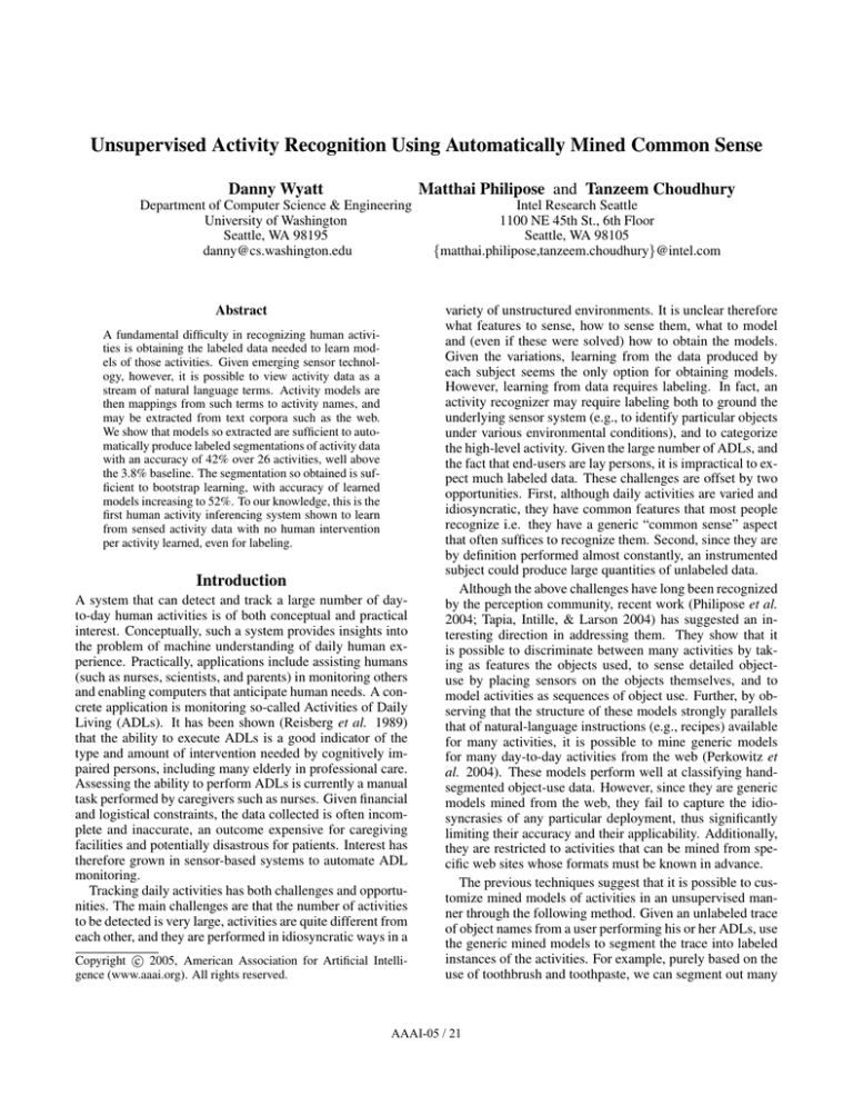
Figure 1: Sensors: RFID reader bracelet (left), RFID tagged
toothbrush and toothpaste (right), tags circled.
web mining approach since we are interested in economically modeling a very wide variety of activities, but focus on
extracting object-use information.
This work improves that of (Perkowitz et al. 2004),
which shows that models mined automatically from a single instructional web site are quite good at classifying handsegmented activity data gathered from RFID-based sensors.
Our work shows how to mine improved models of arbitrary
activities from the web as a whole, and how to use the mined
models to learn customized models from unsegmented, unlabeled sensor data.
Sensors
Figure 1 illustrates the RFID infrastructure that we assume.
On the left is a bracelet which has incorporated into it an
antenna, battery, RFID reader and radio. On the right are
day-to-day objects with RFID tags (battery-free stickers that
currently cost 20-40 cents apiece) attached to them. The
reader constantly scans for tags within a few inches. When
the wearer of the bracelet handles a tagged object, the tag on
the object modulates the signal from the reader to send back
a unique 96-bit identifier (ID). The reader can then ship the
tag ID wirelessly to other ambient computing devices which
can map the IDs to object names. We currently assume that
subjects or their caregivers will tag objects; we have tagged
over a hundred objects in a real home in a few hours. In the
future it is conceivable that the tags will be integrated into
objects by their manufacturers, as barcodes are today. The
infrastructure is the same as that in (Perkowitz et al. 2004),
except that we have replaced the glove required in that work
with a bracelet, a step crucial for acceptance in the ADL
application.
Mining Models from the Web
Given a set of activities A, we seek to mine from the web
a set of objects O used for each activity a in A and their
associated usage probabilities p(o ∈ O|a ∈ A). Our mining proceeds in four distinct steps. First, for each activity
in A, we identify web pages that describe that activity being
performed. Second, having identified these pages, we then
extract from the pages phrases that describe the objects used
during the performance of the activity. Third, once the set of
pages and phrases have been found, co-occurrence statistics
for the pages and phrases are used to estimate the object-use
AAAI-05 / 22
probabilities. Finally, we use the mined information to assemble a Hidden Markov Model (HMM) capable of recognizing activities in traces of object data. Each of these steps
is described in more detail in the subsections below.
Altogether, the mining process corresponds to the intuition that textual descriptions of human activities reflect realworld performances of those activities, both in contents and
statistics.
Identifying pages describing activity performances
In order to identify the objects used in an activity it is not
sufficient to find only the pages that mention the activity,
but rather the subset of those pages that contain detailed descriptions of the activity being performed. Specifically, we
seek only pages that provide instructions on how to perform
an activity. Identifying this subset is a problem known as
genre classification. Genre classification is different than
traditional topical text classification in that it attempts to
determine a document’s genre independently of the document’s topic (Karlgren & Cutting 1994; Kessler, Numberg,
& Schütze 1997; Dewdney, VanEss-Dykema, & MacMillan
2001). Where topic is the subject of the document, genre
is the type of information provided about the topic. For example, in our case, the genre of the documents we want is
“instructional” or “how-to’s”, while the topic of a document
is the activity for which the document provides instructions.
The first step in our genre discrimination is to use a search
engine and its ranking function to identify an initial set of
candidate pages by querying for the activity name combined
with a genre discriminating phrase. We use Google as our
search engine and “how to” as our discriminating phrase.
We retrieve P , the top z pages returned by the search engine
for our query, and seek to find Pe, the subset of P containing only pages in the instructional genre. The simplest approach, of course, is to assume that P = Pe, but we achieved
better recognition accuracy by building a specialized genre
classifier that further refined P .
We experimented with a variety of text features and three
classification algorithms (C4.5, Naive Bayes, and Support
Vector Machines), measuring their performance only in
terms of their classification accuracy. We used a training
set of 352 labeled web pages, evenly divided between positive and negative examples, and a test set of 100 labeled
pages (also evenly split). This is the only supervision that
our system requires. The SVM performed best, with a feature vector comprising TF-IDF (Manning & Schütze 1999)
scores for the top 1,000 words in the corpus as well as (after
(Finn & Kushmerick 2003)) normalized counts of the parts
of speech appearing in a document. When applying the classifier to a set of new pages, we compute the top 1,000 words
across both the 352 training examples as well as the pages
in the new set and then retrain the classifier using the newly
constituted feature vectors of the training data.
Identifying objects
For each page p in Pe, we identify the set of objects mentioned in p. To identify the terms that denote objects, we
must ensure that the terms identified are used as nouns (e.g.
the verb sense of “pan” is excluded), that the nouns identified are tangible objects or substances (e.g. “corporation” is excluded), and that noun modifiers are maintained
when appropriate (e.g. “paper towel” is extracted as a single term). To this end, we tokenize each page into sentences, tag each word in a sentence with its part of speech
(POS), and then chunk each sentence into its constituent
phrases. Then, we take only the noun phrases from the
page and trim each noun phrase to at most its four final
nouns. We then iteratively remove leading nouns until we
find a phrase that is categorized as an object or substance in
WordNet (Fellbaum 1998). We call this phrase an extraction. For each extraction of object oi in page p, we compute a score wi,p = p(object|noun)p(noun)—the probability that the extraction denotes a physical object. p(noun)
is the probability (assigned by the POS tagger) that the last
word of the phrase has noun as its POS. For each sense of
a word, WordNet contains usage counts from a sample corpus. We use these statistics to compute p(object|noun) =
# occurrences of noun senses categorized as objects or substances
. By
# occurrences of all noun senses
deriving this extraction weight from a distribution over word
senses, we avoid having to disambiguate a word’s sense
while favoring (literally) the common sense. Note that since
each object can be extracted multiple times from a single
page and each extraction has its own weight, it is possible
for a single object to have several weights on one page. We
use the mean of these weights as the aggregate score, ŵi,p ,
for object oi on page p.
Computing object use probability
We set the probability p(oi |a) =
1
e|
|P
P
p
ŵi,p —the fraction
of pages in which oi appears, weighted by its average extraction score on each page. For comparison, we also consider the unweighted fraction (setting all ŵi,p = 1), and
the Google Conditional Probability (Perkowitz et al. 2004),
activity)
, where hitcount(q) is the
GCP(oi ) = hitcount(object
hitcount(activity)
number of pages returned as matches for the query q.
Assembling the models
From the mined information, we assemble an HMM, M ,
that has the traditional 3 parameters: the prior probabilities
for each state π, the transition probability matrix T , and the
observation probability matrix B. We define one state for
each activity in A and use the set of objects mined (or a
subset of it) as the set of observations.
We set the observation probabilities to normalized values
of the mined probabilities: Bji = p(oi |aj ). π is set to a uniform distribution over activities. For T , we assume an expected duration γ for any activity and set all self-transition
probabilities Tjj = 1− γ1 . We distribute the remaining probability mass uniformly over all transitions to other activities.
γ can be set based on observational evidence or to a value
that maximizes the likelihood of some training data. Since
we want to learn our model without supervision, we set γ to
an initial value of 5 for all of our experiments. Subsequent
experiment revealed accuracy to be robust across many values of γ.
AAAI-05 / 23
Learning with the Mined Model
Given a set E of unlabeled traces (a trace is a sequence of
names of sensed objects), we can use our mined model as a
basis for learning a model customized for the person or persons who produced E. To train this customized model from
the generic model M , we first apply the Viterbi algorithm to
find the Maximum a Posteriori labeling of E according to
M . We then compute the Maximum Likelihood (ML) observation probabilities according to the labeled trace. For all
states that appear in the labeled trace, we replace their observation probabilities with the learned ML probabilities. For
states that do not appear in the labeled trace we leave their
observation probabilities set to the mined probabilities.
Ranking Segmentation and Grouping
Classification Results
Accuracy may not be what all applications using the segmentation require. In particular, for some applications it
may be useful to increase the precision of the classification by only selecting those examples that are labeled
with high confidence. To this end, we compute a confidencepscore c for a labeled segment (aj , o1 . . . on ) as
Qn
c = n πj p(o1 |aj ) i=2 p(oi |aj )Tjj , which is essentially
the likelihood that the observations o1...n were generated
by a length-n path starting in state aj and self-transitioning
n − 1 times. We normalize this likelihood for the length of
the segment by taking the geometric mean. We expect that
segments that are faithful to the model will have high values
of c. Given a confidence threshold tc , we can return only
those segments with c > tc . Higher values of tc will therefore increase precision (the fraction of classifications that
are correct), typically at the expense of recall (the fraction
of correct classifications returned).
In some cases, an application may be content with a classification that puts a particular segment into a class of a
few “similar” activities, such as “cleaning the kitchen” and
“cleaning the microwave”. If the system is able to provide
sufficient resolution, then it can increase its accuracy since it
no longer needs to distinguish between these similar activities.
Under our model, activities are characterized as distributions over objects. Thus, any technique for comparing probability distributions can be used to compare activities. We
use the Kullback-Leibler (KL) divergence between two activities aj and ak as a measure of the similarity of ak to aj .
Given a similarity threshold ts , if a model extracts a segment
with label aj , then we also declare the segment to be a match
for all activities a0 that are within a KL-distance ts from aj .
Evaluation Methodology
Our evaluation seeks to understand whether:
• Our model mining techniques work. Can we indeed use
mined models to segment and label real activity trace data
with significant accuracy?
• Bootstrapping learning with the segments labeled by the
mined models works. Are the new models we learn significantly more accurate than the mined ones?
• Our selectivity (ranking and grouping) measures work.
How do precision and recall trade off when we vary parameter tc ? Are the activity groupings produced by varying
ts intuitive?
• Various aspects of our design (techniques and parameter
values) had impact. How much do the steps in model
mining contribute, and how do they compare to simpler
approaches? How does the choice of self-transition affect
performance?
For activity traces, we used data from a deployment of
over 100 RFID tags deployed in a real home. The data was
collected well before the current work was initiated. Objects as diverse as faucets and remote controls were tagged.
The data was collected over a period of six weeks, but each
subject took a single 20 to 40 minute session to generate
their data. We had 9 non-researcher subjects with a wearable
RFID reader perform, in any order of their choice, 14 ADLs
each from a possible set of 65; in practice they restricted
themselves to the 26 activities listed in Table 1. The subjects were instructed to perform the activities consecutively,
to avoid interleaved activities. They kept a written log of the
order in which they performed the tasks; we used this log
and perusal of the data stream to establish the ground truth
for our experiments. Each subject produced a trace of observations (tag readings), which we recorded and analyzed
offline. To establish ground truth, we segmented and labeled
the data by hand; in particular, we labeled each observation in the incoming traces with the activity that generated
it. These manual labels are only used for evaluation.
Unfortunately, it is not feasible to perform a direct comparison to the earlier techniques from (Perkowitz et al.
2004). We defer such comparison to a more comprehensive study. Those techniques sought to create activity models with multiple states per activity and then evaluated those
models on traces that were hand-segmented into single activity episodes. Additionally, because their models were mined
from a single web site they had to manually map their models to the activities found in their data (sometimes mapping
multiple mined activities to a single true activity) as well as
map mined object names to tag names. Our method has a
strict one-to-one match between mined activity models and
true activities, and because we discover far more objects per
activity we do not need to map any tag names to mined
names. Our system requires no additional input beyond the
natural language names of activities and tags.
Results
Efficacy of Mining and Learning To test our mining
techniques, we used the composite mined model to segment
and label the 9 traces. We define the overall accuracy of
the trace as the number of observations whose inferred label matched ground truth (true positives, nt , divided by the
total number of observations N ). We define the accuracy
with respect to each activity aj as nt,j /Nj , where nt,j is
the number of observations inferred correctly to have been
generated by activity aj , and Nj is the total number of observations hand-attributed to aj .
AAAI-05 / 24
a
b
c
d
e
f
g
h
i
j
k
l
m
adjust thermostat
boil water in the microwave
brew a pot of tea
brush your hair
brush your teeth
change a baby’s diaper
clean a toilet
clean the bathroom
clean the kitchen
do laundry
dress a baby
drink water
load and run a dishwasher
n
o
p
q
r
s
t
u
v
w
x
y
z
make a peanut butter and
jelly sandwich
make a snack
play solitaire
put on make up
read a magazine
shave your face
take vitamins
use microwave
use the telephone
use toilet
vacuum carpets and floors
wash your hands
watch tv
Table 1: Activities performed
1
0.8
0.6
0.4
0.2
0
a b c d e f g h i j k l m n o p q r s t u v w x y z All
Figure 2: Per activity accuracies, mined (left) vs. learned
(right) models. Letters correspond to Table 1.
To test our learning techniques, we used leave-one-out
cross validation. We first segmented and labeled the traces
using the mined models. We then successively left out one
of the nine traces, used the remaining eight to learn new activity models, and then labeled the left out trace using the
learned models. At the end of this process, we counted correct labels for each left-out trace and calculated overall and
per-activity accuracy as before.
Since each trace comes from a different user, the learned
model is not customized to a single individual. Rather, it is
customized to the environment—the set of available objects.
This is akin to learning a model for a specific household.
Liao, Fox, & Kautz (2005) have shown that learning models
from different individuals can improve activity recognition
for a new individual, and we expect accuracy to improve
even more for the case where all of the training data comes
from a single person.
Figure 2 summarizes the results. The rightmost pair of
bars compares the overall accuracy of the mined models
(left bar) and learned models (right bar). With purely mined
models, we achieve an accuracy of 42%. With learning,
accuracy goes up to 52%. Two limits are worth noting
here. First, given that we have 26 activities, random labeling would achieve roughly 3.8% accuracy. Thus, both mined
and learned models are quite strong predictors. Further, even
with the modest amount of unlabeled data to learn from (it
is not unreasonable to posit that a future system could have
many hundreds of instances of each activity), the learning
can improve significantly upon the commonsense models.
Second, when we used the manual labels to learn a model
from the traces and tested it on the same traces (again using
leave-one-out validation), we achieved an accuracy of 73%.
The performance of unsupervised, mined-model labeling is
thus not too far from that of supervised labeling.
Although learned accuracy is better than mined accuracy
for most activities, it is worse in some cases. This is partly
because accuracy is sometimes gained at the cost of precision, and partly because in some cases we do not have much
data on which to learn. In the case of solitaire, for example, these two factors combine: the traces contain only one
instance of playing solitaire, and the mined models imprecisely label a number of segments (including half the observations in the correct one) as solitaire. The mined model
thus gets a 50% score, whereas the learned model (biased towards the incorrect examples produced) gets a zero. To mitigate bad examples, we attempted to use for learning only
examples with high confidence; unfortunately, this resulted
in worse results after learning. Essentially, filtering results
in even fewer good examples getting to the learner. On examining the data, we believe that although not filtering allows many more bad examples to be input to the learner,
the bad ones are much less correlated than the good ones.
Of course, with sufficient unlabeled data, even restricting to
high-confidence examples will yield enough examples.
Table 2 shows the complete 26×26 confusion matrix. The
entry in row i, column j represents the number of times an
observation with ground truth label i was labeled as activity j. The numbers in parentheses are counts for the learned
model, where they differ from the mined models; numbers
for the latter are not parenthesized. Three points are worth
nothing. First, the diagonal numbers for the learned matrix
are significantly better than for the mined ones. Second, the
off-diagonal behavior does not show a discernible trend: the
learned models do not systematically avoid certain confusions. Finally, the problem mentioned above with playing
solitaire is illustrated: we have many more false positives
than true ones.
Efficacy of Selectivity Parameters Figure 3 shows how
effective the confidence threshold tc is in trading off precision for recall over all activities when labeling and thresholding is performed with the mined models alone, the
learned models alone, and a combination of learned and
mined models. Recall that when confidence thresholding is
enabled, we only classify as a match those segments labeled
with confidence greater than tc . Precision in this context
is therefore the ratio of the number of correct classifications
that are above threshold to the total number of classifications
above threshold. Recall is the ratio of the number of correct
classifications above threshold to the total number of correct
classifications we produce. The lower the recall, the more
correct classifications we “waste”.
The figure shows that thresholding on label likelihood has
mixed results. With mined models, it is indeed possible to
trade off precision for recall by varying tc . For instance, it is
possible to achieve 70% precision while only “wasting” 30%
of our correct classifications. Unfortunately, the case for us-
AAAI-05 / 25
a
b
c
d
e
f
g
h
i
j
k
l
m
n
o
p
q
r
s
t
u
v
w
x
y
z
a
8(8)
0
1(1)
3(4)
8
1
2(2)
0
0
0
0
0
0
0
0
0
0
0
1(1)
0
0
1
15(12)
2
0
0
b
0
5(2)
8(5)
0
0
0
0
0
0
0
0
3
0(2)
0
0
0
0
0
0
4(2)
4(5)
0
0
0
0
0
c
0
0
1(4)
0
0
0
0
0
0
0
0
0
0
0
0
0
0
0
0
0
0
0
0
0
0
0
d
0
0
0
4(11)
15(7)
0
0
0
0
0
0
0
0
0
0
0
7(10)
0
0
0
0
0
0
0
4(2)
0
e
0
0
0
0
12(12)
0
0
0
0
0
0
0
0
0
0
0
0
0
0
0
0
0
0
0
0
0
f
0
0
0
0
0
31(33)
0
0
0(1)
0
0
0
0
0
0
0
0
0
0
0
0
0
0
0
0
0
g
0
0
0
0
0
0
0
0
0
0
0
0
0
1
3
0
1
2
0
0
0
13
4
0
0
0
h
0
3(8)
4(4)
0
8(16)
0
0(3)
15(15)
9(4)
0(2)
3(3)
13(5)
0
0
0
0
0
0
1
3
0
0
0
0
0
0
i
0
2
0
0
0
0
0
0
4(13)
0
0
3(13)
0
4(1)
14(17)
0
0
0
0
0
0
1
0
0
0
0
j
0
0
0
0(1)
0
0
0
0
0
8(7)
0
0
0
0
0
0
0
0
0
0
0
0
1
0
0
0
k
0
0
0
0
0(1)
17(17)
0
0
0
0
19(19)
0
0
0
0
0
0
0
0
0
0
0
0
0
0
0
l
0
0
0
0
0
0
0
0
0
0
0
1
0
0
0
0
0
0
0
11(14)
0
0
0
0
0
0
m
1(1)
0
0
8
4(4)
0
7(3)
0
0
21(20)
0
0
16(14)
11(3)
0
0
0
0
0
0
1(1)
0
8
1(3)
5(6)
0
n
0
0
0
0
0
0
0
0
0
0
0
0
0
31(45)
3(1)
0
0
0
0
0
0
0
0
0
0
0
o
0
0
0
0
0
0
0
0
0
0
0
0
0
2(5)
0
0
0
0
0
0
0
0
0
0
0
0
p
0
0
0
0(2)
14(22)
0
0
0
0
0
0
0
0
0
0
2
0
0(1)
0
0
0
0
0(1)
0
5(8)
0
q
0
0
0
0
0
0
0(1)
0
0
0
0
0(2)
0
0
0
0(4)
0
0
0
0
0
0
0
0
0
0
r
0
0
0
0
0
0
0
0
0
0
0
0
0
0
0
0
0
0(1)
0
0
0
0
0
0
0
0
s
0
0
0
0(2)
0
0
0
0
0
0
0
0
0
0
0
0
0
0
20(21)
0
0
0
1
0
0
0
t
0
0
0
0
0
0
0
0
0
0
0
0
0
0
0
0
0
0
0
5(5)
0
0
0
0
0
0
u
0
0
0
0
0
0
0
0
3
0
0
0
0
11(8)
0
0
2
0
0
4(6)
4(3)
0
0
0
0
0
v
0
0
0
0
0
0
0
0
0
0
0
0
0
0
0
0
0
0
0
0
0
10(27)
0
0
0
0
w
0
0
0
0(3)
1
1
0
0
0
0
1(1)
0
0
0
0
0
0
0
0(1)
0
0
3
15(31)
0
5(3)
0
x
0
0
0
8
0
0
0
0
0
0
0
0
0
0
0
0
0
0
0
0
0
0
0
9(9)
0
0
y
0
0
0
0
0
0
0
0
2
0
0
0
0
2
0(2)
0
0
0
1
0
0
0
0
0
0
0
z
0
0
0
0
0
0
0
0
0
0
0
0
0
0
0
2
0
0
0
0
0
11(12)
0
0
0
35(35)
Table 2: Confusion matrix: mined (learned) models. Letters correspond to Table 1.
1
1
0.9
0.9
0.8
0.7
0.7
Accuracy
Precision
0.8
0.6
0.6
0.5
0.4
0.3
0.5
0.2
Mined
Learned, ranked by Mined
Learned
0.4
0
0.1
0.2
0.3
0.4
0.5
Recall
0.6
0.7
0.1
0.8
0.9
0
1
Mined
Learned
0
0.1
0.2
0.3
0.4
0.5
0.6
Baseline
0.7
0.8
0.9
1
Figure 3: Precision and recall for varying tc
Figure 4: Accuracy vs. baseline for varying ts
ing tc to control the trade-off is no longer as strong when the
threshold is computed using learned models: the P/R curve
is flatter, and it has a precipitous dip on the left which we
cannot currently explain. An interesting compromise may
be to segment with the learned model, then rank the segments so obtained using the mined models (which seem to
have good separation properties). As the figure shows, this
hybrid solution allows us to trade off precision and recall
well on learned-model-segmented data.
Figure 4 shows how effective the similarity threshold ts
is in trading off accuracy (y-axis) for resolution (x-axis).
Recall that increasing ts groups activities into increasingly
larger classes, and classification is over these classes. Since
the classifier has to distinguish between fewer classes, it
should become increasingly accurate. Of course, having
fewer classes implies that random guessing would also do
better. This average accuracy may be viewed as an inverse
measure of “resolution”: high baseline accuracy implies
fewer classes distinguishable. Instead of charting how accuracy changes with ts , therefore, we find the new classes for
each new value of ts , calculate the baseline accuracy for this
class, and plot overall accuracy vs. baseline accuracy. Accuracy rises fairly quickly at low values of ts , indicating that
KL-distance may be a good metric for grouping activities.
It is possible, for instance, to achieve 80% overall accuracy
when random guessing would only achieve 20%. More qualitatively, the system is quite successful at grouping “similar”
activities. For instance, setting ts to 1 groups “brew a pot of
tea” with “boil water in a microwave”, “wash your hands”
with “use the toilet”, and (perhaps more questionably) “use
the toilet” with “clean the toilet”.
Impact of Web Mining and Parameter Choices To determine whether some of the more sophisticated aspects of
our web-mining scheme are warranted, we performed four
experiments comparing overall activity recognition accuracy. (1) We compared models generated using all 50 pages
AAAI-05 / 26
returned by Google, using only the n returned by the genre
classifier, and using a random size n subset of the 50 pages.
(2) We compared using all tagged nouns that are substances
or objects to using noun-phrase-based extractions. (3) We
compared using the extraction-weight based probability of
object use to unweighted probabilities and Google Conditional Probabilities. (4) We compared using only objects
found in the incoming data to using the union of the top 100
most likely objects from each activity.
We found that in each experiment, the more sophisticated
technique had a consistent and noticeable benefit. In each
case below, we fix all other parameters so as to obtain the
best result for the parameter being varied. (1) At best, using
all 50 pages yields 50% accuracy, a random n gave 42% and
the genre classifier gave 52%. (2) Using noun-phrase-based
extractions gives 52% accuracy, not doing so gives 47%. (3)
Extraction-weight probabilities give 52%, unweighted give
49%, and GCP gives 48%. (4) Restricting the HMM’s possible observations to only the objects found in the data gives
52%, not doing so 37%. Overall, filtering to the data objects seems to have very high impact; on the other hand,
the engineering overhead of genre classification may not be
worthwhile.
To determine how the choice of self-transition probability affects our results, we calculated accuracies for selftransition probabilities ranging from 0.019 (one half of uniform) to 0.98 in increments of 0.019. For the mined model,
the mean accuracy across these values was 42.7% with a
standard deviation of 2.9%. After learning from these models, mean accuracy was 47.8% with a standard deviation of
4.5%. Thus the self-transition probability does not have a
large effect on the raw accuracy of the mined model, but it
does have a greater effect on learning.
Conclusions
Densely deployable wireless sensors developed in recent
years have made it possible to detect objects used in daily
activities in great detail. Given the names of these objects,
it is possible to infer, with significant accuracy, the activity
currently being performed. We demonstrate that, for a very
large class of day-to-day activities (those characterized by
objects used), it is possible to automatically and simply mine
models from the web. The mined models are themselves
quite accurate, but more interestingly, they can be used to
segment unlabeled data and thereby bootstrap sensor-based
customization of the models. Even with modest amounts of
unlabeled data, the customized models are much more accurate than the mined ones. Measures based on the similarity
between the models and the likelihood of segments may be
used to trade off precision, recall, accuracy and resolution of
classification.
References
Blum, A., and Mitchell, T. M. 1998. Combining labeled and
unlabeled data with co-training. In Proceedings of COLT, 92–
100.
Brill, E.; Lin, J. J.; Banko, M.; Dumais, S. T.; and Ng, A. Y. 2001.
Data-intensive question answering. In Proceedings of the Tenth
Text REtrieval Conference.
Craven, M.; DiPasquo, D.; Freitag, D.; McCallum, A.; Mitchell,
T. M.; Nigam, K.; and Slattery, S. 1998. Learning to extract
symbolic knowledge from the world wide web. In Proceedings of
AAAI-98, 509–516.
Dewdney, N.; VanEss-Dykema, C.; and MacMillan, R. 2001. The
form is the substance: Classification of genres in text. In Proceedings of the ACL 2001 Workshop on Human Language Technology
and Knowledge Management.
Etzioni, O.; Cafarella, M.; Downey, D.; Popescu, A.-M.; Shaked,
T.; Soderland, S.; Weld, D. S.; and Yates, A. 2004. Methods
for domain-independent information extraction from the web: An
experimental comparison. In Proceedings of AAAI-04, 391–398.
Fellbaum, C. 1998. WordNet An Electronic Lexical Database.
Boston: MIT Press.
Fernyhough, J. H.; Cohn, A. G.; and Hogg, D. 2000. Constructing
qualitative event models automatically from video input. Image
and Vision Computing 18(2):81–103.
Finn, A., and Kushmerick, N. 2003. Learning to classify documents according to genre. In IJCAI-03 Workshop on Computational Approaches to Style Analysis and Synthesis.
Guyon, I., and Elisseeff, A. 2003. An introduction to variable and
feature selection. Journal of Machine Learning Research 3:1157–
1182.
Karlgren, J., and Cutting, D. 1994. Recognizing text genres with
simple metrics using discriminant analysis. In Proceedings of
COLING 94.
Kessler, B.; Numberg, G.; and Schütze, H. 1997. Automatic
detection of text genre. In Proc. of the 35th conference of the
Association for Computational Linguistics, 32–38. ACL.
Lenat, D. B., and Guha, R. V. 1990. Building Large KnowledgeBased Systems: Representation and Inference in the CYC Project.
Reading, Massachusetts: Addison-Wesley.
Lewis, D. D., and Gale, W. A. 1994. A sequential algorithm for
training text classifiers. In Proceedings of SIGIR-94, 3–12.
Liao, L.; Fox, D.; and Kautz, H. 2005. Location-based activity
recognition using relational markov networks. In Proceedings of
the International Joint Conference on Artifical Intelligence (IJCAI).
Manning, C. D., and Schütze, H. 1999. Foundations of Statistical
Natural Language Processing. Cambridge, Massachusetts: The
MIT Press.
Perkowitz, M.; Philipose, M.; Fishkin, K. P.; and Patterson, D. J.
2004. Mining models of human activities from the web. In Proceedings of WWW-04, 573–582.
Philipose, M.; Fishkin, K.; Perkowitz, M.; Patterson, D.; Kautz,
H.; and Hahnel, D. 2004. Inferring activities from interactions
with objects. IEEE Pervasive Computing Magazine 3(4):50–57.
Reisberg, B.; Ferris, S.; deLeon, M.; Kluger, A.; Franssen, E.;
Borenstein, J.; and Alba, R. 1989. The Stage Specific Temporal
Course of Alzheimer’s Disease: Functional and Behavioral Concomitants Based Upon Cross-Sectional and Longitudinal Observation. Progress in Clinical and Biological Research 317:23–41.
Singh, P.; Lin, T.; Mueller, E. T.; Lim, G.; Perkins, T.; and Zhu,
W. L. 2002. Open mind common sense: Knowledge acquisition
from the general public. In CoopIS/DOA/ODBASE, 1223–1237.
Tapia, E. M.; Intille, S. S.; and Larson, K. 2004. Activity recognition in the home using simple and ubiquitous sensors. In Pervasive, 158–175.
Thrun, S., and Mitchell, T. 1995. Lifelong robot learning. Robotics and Autonomous Systems 15:25–46.
AAAI-05 / 27