6.262: Discrete Stochastic Processes
4/11/11
Lecture 17: Countable-state Markov chains
Outline:
• Strong law proofs
• Positive-recurrence and null-recurrence
• Steady-state for positive-recurrent chains
• Birth-death Markov chains
• Reversibility
1
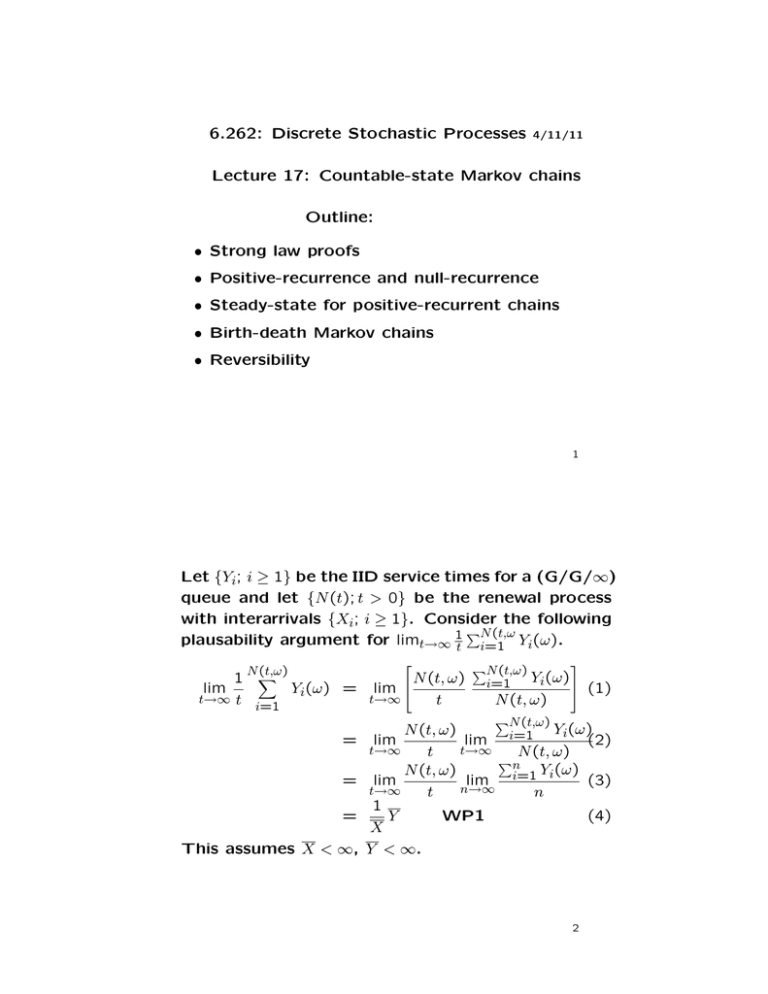
Let {Yi; i ≥ 1} be the IID service times for a (G/G/∞)
queue and let {N (t); t > 0} be the renewal process
with interarrivals {Xi; i ≥ 1}. Consider the following
�N (t,ω
plausability argument for limt→∞ 1t i=1 Yi(ω ).
N�
(t,ω)
1
t→∞ t
i=1
lim


�N (t,ω)
N (t, ω) i=1 Yi(ω) 
Yi(ω) = lim 
(1)
t→∞
t
N (t, ω)
=
=
=
This assumes X < ∞,
�N (t,ω)
Yi(ω)
N (t, ω)
lim
lim i=1
(2)
t→∞
t→∞
t
N (t, ω)
�n
Y (ω)
N (t, ω)
lim
lim i=1 i
(3)
n→∞
t→∞
t
n
1
Y
WP1
(4)
X
Y < ∞.
2
To do this carefully, work from bottom up.
Let A1 = {ω : limt→∞ N (t, ω)/t = 1/X}. By the strong
law for renewal processes Pr{A1} = 1.
�
1 n
Let A2 = {ω : limn→∞ n
By the
i=1 Yi(ω) = Y }.
SLLN, Pr{A2} = 1. Thus (3) = (4) for ω ∈ A1A2
and Pr{A1A2} = 1.
Assume ω ∈ A2, and � > 0. Then ∃m(�, ω) such that
1 �n
|n
i=1 Yi(ω) − Y | < � for all n ≥ m(�, ω). If ω ∈ A1
also, then limt→∞ N (t, ω) = ∞, so ∃t(�, ω) such that
N (t, ω) ≥ m(�, ω) for all t ≥ t(�, ω).
��
�
� N (t,ω)
�
� i=1
�
Y
(ω)
i
�
− Y �� < �
�
N (t, ω)
�
�
for all t ≥ t(�, ω)
Since � is arbitrary, (2) = (3) = (4) for ω ∈ A1A2.
3
Finally, can we interchange the limit of a product of
two functions (say f (t)g(t)) with the product of the
limits? If the two functions each have finite limits
(as the functions of interest do for ω ∈ A1A2), the
answer is yes, establishing (1) = (4).
To see this, assume limt f (t) = a and limt g(t) = b.
Then
f (t)g(t)−ab = (f (t)−a)(g(t)−b) + a(g(t)−b) + b(f (t)−a)
|f (t)g(t)−ab| ≤ |f (t)−a||g(t)−b| + |a||g(t)−b| + |b||f (t)−a|
For any � > 0, choose t(�) such that |f (t) − a| ≤ � for
t ≥ t(�) and |g(t) − b| ≤ � for t ≥ t(�). Then
|f (t)g(t)−ab| ≤ �2 + �|a| + �|b|
Thus limt f (t)g(t) = limt f (t) limt g(t).
for t ≥ t(�).
4
Review - Countable-state chains
Two states are in the same class if they communi­
cate (same as for finite-state chains).
Thm: All states in the same class are recurrent or
all are transient.
Pf: Assume j is recurrent; then
�
n
n Pjj = ∞.
For
m > 0 for some m and P � for
any i such that j ↔ i, Pij
ji
�
some �. Then (recalling limt E [Nii(t)] = n Piin)
∞
�
n=1
Piin ≥
∞
�
k=n−m−�
mP k P � = ∞
Pij
jj jk
By the same kind of argument, if �i ↔ �j are recurrent,
�
n
t
then ∞
n=1 Pij = ∞ (so also limt E Nij = ∞).
5
If a state j is recurrent, then the recurrence time
Tjj might or might not have a finite expectation.
�
�
Def: If E Tjj < ∞, j is positive-recurrent. If Tjj is a
�
�
rv and E Tjj = ∞, then j is null-recurrent. Other­
wise j is transient.
For p = 1/2, each state in each of the following is
null recurrent.
p
q
q
✓✏
−2
②
✒✑
✓✏
✘ 0 ②
✿

✒✑
p
③

q =1−p
p
③

q =1−p
✓✏
−1②

✒✑
✓✏
1 ②

✒✑
p
③

q
p
q
③

✓✏
0 ②

✒✑
✓✏
2 ②

✒✑
p
✗✔
③

p
✖✕
1
q
p
q
✗✔

③
p
✖✕
3
q
q
6
Positive-recurrence and null-recurrence
Suppose i ↔ j are recurrent. Consider the renewal
process of returns to j with X0 = j. Consider re­
wards R(t) = 1 whenever X(t) = i. By the renewalreward thm (4.4.1),
1
lim
t→∞ t
� t
E [Rn]
WP1,
T jj
0
where E [Rn] is the expected number of visits to i
within a recurrence of j. The left side is limt→∞ 1t Nji(t),
which is 1/T ii. Thus
R(τ )dτ =
1
E [Rn]
=
T ii
T jj
Since there must be a path from j to i, E [Rn] > 0.
Thm: For i ↔ j recurrent, either both are positive­
recurrent or both null-recurrent.
7
Steady-state for positive-recurrent chains
We define steady-state probabilities for countablestate Markov chains in the same way as for finitestate chains, namely,
Def: {πi; i ≥ 0} is a steady-state distribution if
πj ≥ 0; πj =
�
i
πiPij
for all j ≥ 0
and
�
πj = 1
j
Def: An irreducible Markov chain is a Markov chain
in which all pairs of states communicate.
For finite-state chains, irreducible means recurrent.
Here it can be positive-recurrent, null-recurrent, or
transient.
8
If steady-state π exists and if Pr{X0 = i} = πi for
�
each i, then pX1 (j) = i πiPij = πj . Iterating, pXn (j) =
� (t) be num­
πj , so steady-state is preserved. Let N
j
ber of visits to j in (0, t] starting in steady state.
Then
�
�
� (t) =
E N
j
n
�
Pr{Xk = j} = nπj
k=1
� (t)
Awkward thing about renewals and Markov: N
j
works for some things and Njj (t) works for others.
Here is a useful hack:
Nij (t) is 1 for first visit to j (if any) plus Nij (t) − 1
for subsequent recurrences j to j. Thus
�
�
E Nij (t)
�
�
� (t)
E N
j
�
�
≤ 1 + E Njj (t)
=
�
i
�
�
�
�
πiE
Nij (t) ≤ 1 + E Njj (t)
9
Major theorem: For an irreducible Markov chain,
the steady-state equations have a solution if and
only if the states are positive-recurrent. If a solution
exists, then πi = 1/T ii > 0 for all i.
Pf: (only if; assume π exists, show positive-recur.)
For each j and t,
�
�
� (t)
E N
j
�
1
+
t �
t�
t
E Njj (t)
1
≤ lim
=
t→∞
t
T jj
πj =
�
≤
�
E Njj (t)
�
�
Since j πj = 1, some πj > 0. Thus limt→∞ E Njj (t) /t >
0 for that j, so j is positive-recurrent. Thus all
states are positive-recurrent. See text to show that
‘≤’ above is equality.
10
Birth-death Markov chains
q0
✓✏
✿ 0 
✘
②
✒✑
❖
p0
③

✓✏
1 
②
✒✑
❖
q1
p1
③

✓✏
p2
2 ②

✒✑
❖
q2
q3

③
✓✏
p3
3
✒✑
❖
For any state i and any sample path, the number
of i → i + 1 transitions is within 1 of the number of
i + 1 → j transitions; in the limit as the length of the
sample path → ∞,
πp
πipi = πi+1qi+1;
πi+1 = i i
qi+1
Letting ρi = pi/qi+1, this becomes
πi = π0
i−1
�
ρj ;
π0 =
j=0
1
.
�∞
�i−1
1 + i=1
j=0 ρj
This agrees with the steady-state equations.
11
q0
✓✏
✿ 0 
✘
②
✒✑
❖
p0
q1
πi = π0
i�
−1
j=0
③

✓✏
1 
②
✒✑
❖
ρj ;
p1
q2
π0 =
③

✓✏
p2
2 
②
✒✑
✗✔
③

p3
✖✕
❖
3
❖
q3
1
.
�∞
�i−1
1 + i=1
ρ
j=0 j
This solution is a function only of ρ0, ρ1, . . . and
doesn’t depend on size of self loops.
The expression for π0 converges (making the chain
positive recurrent) (essentially) if the ρi are asymp­
totically less than 1.
Methodology: We could check renewal results care­
fully to see if finding πi by up/down counting is jus­
tified. Using the major theorem is easier.
Birth-death chains are particularly useful in queuing
where births are arrivals and deaths departures.
12
Reversibility
�
�
�
�
�
Pr Xn+k , ...Xn+1|Xn, ...X0 = Pr Xn+k , ..., Xn+1 | Xn
�
For any A+ defined on Xn+1 up and A− defined on
Xn−1 down,
�
Pr A+ | Xn, A− = Pr A+ | Xn
�
�
�
�
�
�
�
Pr A+, A− | Xn = Pr A+ | Xn Pr A− | Xn .
�
�
�
�
Pr A− | Xn, A+ = Pr A− | Xn .
�
�
Pr Xn−1 | Xn, Xn+1, . . . , Xn+k = Pr{Xn−1 | Xn} .
13
By Bayes,
Pr{Xn | Xn−1} Pr{Xn−1}
.
Pr{Xn}
If the forward chain is in steady state, then
Pr{Xn−1 | Xn} =
Pr{Xn−1 = j | Xn = i} = Pjiπj /πi.
Aside from the homogeniety involved in starting at
time 0, this says that a Markov chain run backwards
is still Markov. If we think of the chain as starting
in steady state at time −∞, these are the equa­
tions of a (homogeneous) Markov chain. Denot­
ing Pr{Xn−1 = j | Xn = i} as the backward transition
∗ , forward/ backward are related by
probabilities Pji
∗ =π P .
πiPij
j ji
∗ = P for all i, j.
Def: A chain is reversible if Pij
ij
14
Thm: A birth/death Markov chain is reversible if it
has a steady-state distribution.
✲
�
✟�
✟✟
✟
✟
✟
�
�
�
✟�
✟✟
✟
✟
�
✟
✛
�
�
�❍
❍
❍❍
❍❍�
�
�
�
�
�
δ
✲
�
�
�
✟�
✟
Arrivals
✟✟
✟
✟
�
�
�
�
✟✟
✟✟
✟
✲
�
✟✟
✟✟
✟
✟
✟
�
Departures
✟�❍
❍
✟✟
❍❍
✟
❍❍�
� ✟
✟
❍❍
❍
❍❍
❍�
State
�
�
❍
❍❍
✛
❍❍
✛
❍�
�❍
❍
❍❍
❍❍
❍❍
❍
❍❍�
❍�
�
Arrivals
Departures
15
MIT OpenCourseWare
http://ocw.mit.edu
6.262 Discrete Stochastic Processes
Spring 2011
For information about citing these materials or our Terms of Use, visit: http://ocw.mit.edu/terms.