6.262: Discrete Stochastic Processes
3/28/11
Lecture 14: Review
The Basics: Let there be a sample space, a set of
events (with axioms), and a probability measure on
the events (with axioms).
In practice, there is a basic countable set of rv’s
that are IID, Markov, etc.
A sample point is then a collection of sample values,
one for each rv.
There are often uncountable sets of rv’s, e.g., {N (t); t ≥
0}, but they can usually be defined in terms of a ba­
sic countable set.
1
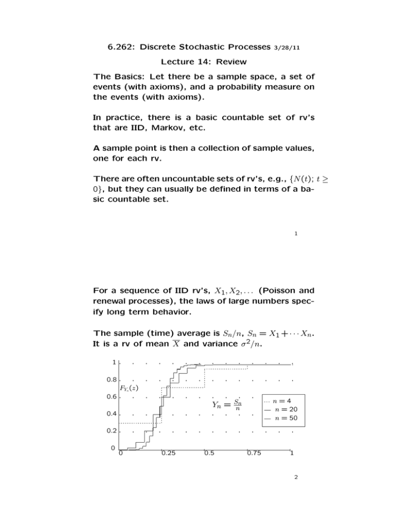
For a sequence of IID rv’s, X1, X2, . . . (Poisson and
renewal processes), the laws of large numbers spec­
ify long term behavior.
The sample (time) average is Sn/n, Sn = X1 + · · · Xn.
It is a rv of mean X and variance σ 2/n.
1·
·
·
·
·
·
·
·
·
·
·
·
·
0.8 ·
·
FYn (z)
0.6 ·
·
·
·
·
·
·
·
·
·
·
·
·
·
·
·
·
·
·
·
0.4 ·
·
·
·
·
·
·
· · ·
Yn = Snn
· · ·
·
0.2
·
·
·
·
·
·
·
·
·
0
0
·
0.25
0.5
·
·
0.75
n=4
n = 20
n = 50
·
·
·
1
2
The weak LLN: If E [|X|] < ∞, then
�
��
�
� Sn
�
�
�
lim Pr �
− X� ≥ � = 0
for every � > 0.
n→∞
n
�
�
This says that Pr Snn ≤ x approaches a unit step
at X as n → ∞ (Convergence in probability and in
distribution).
The strong LLN: If E [|X|] < ∞, then
Sn
lim
=X
n→∞ n
W.P.1
This says that, except for a set of sample points of
zero probability, all sample sequences have a limiting
sample path average equal to X.
Also, essentially limn→∞ f (Sn/n) = f (X) W.P.1.
3
There are many extensions of the weak law telling
how fast the convergence is. The most useful re­
sult about convergence speed is the central limit
2 < ∞, then
theorem. If σX
�
�
Sn − nX
lim Pr
≤y
√
n→∞
nσ
��
Equivalently,
�
�
��
� y
�
�
� y
�
�
1
−x2
√ exp
=
2
−∞ 2π
dx.
1
−x2
√ exp
=
dx.
2
−∞ 2π
√
In other words, Sn/n converges to X with 1/ n and
becomes Gaussian as an extra benefit.
Sn
yσ
lim Pr
−X ≤ √
n→∞
n
n
4
Arrival processes
Def: An arrival process is an increasing sequence
of rv’s, 0 < S1 < S2 < · · · . The interarrival times are
X1 = S1 and Xi = Si − Si−1, i ≥ 1.
X3
✛
✛
✛
X1
0
X2 ✲
✲
S1
✲
✻
N (t)
t
S2
S3
An arrival process can model arrivals to a queue,
departures from a queue, locations of breaks in an
oil line, etc.
5
X3
✛
✛
✛
0
X1
X2 ✲
✲
S1
✲
✻
N (t)
t
S2
S3
The process can be specified by the joint distribu­
tion of either the arrival epochs or the interarrival
times.
The counting process, {N (t); t ≥ 0}, for each t, is
the number of arrivals up to and including t, i.e.,
N (t) = max{n : Sn ≤ t}. For every n, t,
{Sn ≤ t} = {N (t) ≥ n}
Note that Sn = min{t : N (t) ≥ n}, so that {N (t); t ≥ 0}
specifies {Sn; n > 0}.
6
Def: A renewal process is an arrival process for
which the interarrival rv’s are IID. A Poisson process
is a renewal process for which the interarrival rv’s
are exponential.
Def: A memoryless rv is a nonnegative non-deterministic
rv for which
Pr{X > t+x} = Pr{X > x} Pr{X > t}
for all x, t ≥ 0.
This says that Pr{X > t+x | X > t} = Pr{X > x}. If
X is the time until an arrival, and the arrival has
not happened by t, the remaining distribution is the
original distribution.
The exponential is the only memoryless rv.
7
Thm: Given a Poisson process of rate λ, the interval
from any given t > 0 until the first arrival after t is
a rv Z1 with FZ1 (z) = 1 − exp[−λz]. Z1 is independent
of all N (τ ) for τ ≤ t.
Z1 (and N (τ ) for τ ≤ t) are also independent of fu­
ture interarrival intervals, say Z2, Z3, . . . . Also {Z1, Z2,
. . . , } are the interarrival intervals of a PP starting
at t.
The corresponding counting process is {Ñ (t, τ ); τ ≥
t} where Ñ (t, τ ) = N (τ ) − N (t) has the same distribu­
tion as N (τ − t).
This is called the stationary increment property.
8
Def: The independent increment property for a
counting process is that for all 0 < t1 < t2 < · · · tk ,
the rv’s N (t1), [Ñ (t1, t2)], . . . , [Ñ (tn−1, tn)] are indepen­
dent.
Thm: PP’s have both the stationary and indepen­
dent increment properties.
PP’s can be defined by the stationary and indepen­
dent increment properties plus either the Poisson
PMF for N (t) or
�
�
Pr Ñ (t, t+δ) = 1
= λδ + o(δ)
Pr Ñ (t, t+δ) > 1
= o(δ).
�
�
9
The probability distributions
fS1,... ,Sn (s1, . . . , sn) = λn exp(−λsn)
for 0 ≤ s1 ≤ · · · ≤ sn
The intermediate arrival epochs are equally likely to
be anywhere (with s1 < s2 < · · · ). Integrating,
λntn−1 exp(−λt)
Erlang
(n − 1)!
The probability of arrival n in (t, t + δ) is
fSn (t) =
Pr{N (t) = n−1} λδ = δfSn (t) + o(δ)
f (t)
Pr{N (t) = n−1} = Sn
λ
(λt)n−1 exp(−λt)
=
(n − 1)!
(λt)n exp(−λt)
Poisson
pN (t)(n) =
n!
10
Combining and splitting
If N1(t), N2(t), . . . , Nk (t) are independent PP’s of rates
�
λ1, . . . , λk ,then N (t) = i Ni(t) is a Poisson process of
�
rate j λj .
Two views: 1) Look at arrival epochs, as generated,
from each process, then combine all arrivals into
one Poisson process.
(2) Look at combined sequence of arrival epochs,
then allocate each arrival to a sub-process by a se­
�
quence of IID rv’s with PMF λi/ j λj .
This is the workhorse of Poisson type queueing
problems.
11
Conditional arrivals and order statistics
n!
fS� (n)|N (t)(�s(n) | n) = n
t
for 0 < s1 < · · · sn < t
�
�
t−τ n
Pr{S1 > τ | N (t)=n} =
t
�
for 0 < τ ≤ t
�
t−τ n
Pr{Sn < t − τ | N (t)=n} =
for 0 < τ ≤ t
t
The joint distribution of S1, . . . , Sn given N (t) = n is
the same as the joint distribution of n uniform rv’s
that have been ordered.
12
Finite-state Markov chains
An integer-time stochastic process {Xn; n ≥ 0} is a
Markov chain if for all n, i, j, k, . . . ,
Pr{Xn = j | Xn−1=i, Xn−2=k . . . X0=m} = Pij ,
where Pij depends only on i, j and pX0 (m) is arbitrary.
A Markov chain is finite-state if the sample space
for each Xi is a finite set, S. The sample space S
usually taken to be the integers 1, 2, . . . , M.
A Markov chain is completely described by {Pij ; 1 ≤
i, j ≤ M} plus the initial probabilities pX0 (i).
The set of transition probabilities {Pij ; 1 ≤ i, j ≤
M}, is usually viewed as the Markov chain with pX0
viewed as a parameter.
13
A finite-state Markov chain can be described as a
directed graph or as a matrix.
✎☞
2②

✟✍✌
✯
✟
11
✟✟
✟
✟✟
✎ ✟✟
✎☞
12
1

❍
✍✌
❍❍
44
❍❍
❍❍
❍
41
✎☞
❍✎
P
P23
P32
P
4
✍✌
P63
P45
✎☞
6✌
✍
✡
✡
✡
✡
65✡
✡
✡
55
✡☞
☞
✎✡
✢
✘
✘
✲5②

✍✌
✌
P
P
P
③
✎☞
✛
3✌
✍
a) Graphical
P

P11 P12
 P21 P22
[P ] = 
...
 ...
P61 P62

···
P16
P26 
···
... ... ... ... 

···
P66
b) Matrix
An edge (i, j) is put in the graph only if Pij > 0,
making it easy to understand connectivity.
The matrix is useful for algebraic and asymptotic
issues.
14
Classification of states
An (n-step) walk is an ordered string of nodes (states),
say (i0, i1, . . . in), n ≥ 1, with a directed arc from im−1
to im for each m, 1 ≤ m ≤ n.
A path is a walk with no repeated nodes.
A cycle is a walk in which the last node is the same
as the first and no other node is repeated.
✎☞
2
②
✯✍✌
✟
✟
✟
11
✟
✟
✟
✟✟
✎✟
☞
✎
P
P23
P32
P12
1
❍
✍✌
❍❍
44
❍❍
❍❍
41 ❍❍✎✎ ☞
4
✍✌
P63
P45
✎☞
6
✍✌
✡
✡
✡
✡
65✡
✡
✡
55
✡☞
☞
✎✡
✢
✘
✲5✘

②
✍✌
✌
P
P
P

③✎☞
✛
3✌
✍
P
Walk: (4, 4, 1, 2, 3, 2)
Walk: (4, 1, 2, 3)
Path: (4, 1, 2, 3)
Path: (6, 3, 2)
Cycle: (2, 3, 2)
Cycle: (5, 5)
A node j is accessible from i, (i → j) if there is a
n > 0 for some n > 0.
walk from i to j, i.e., if Pij
15
If (i → j) and (j → k) then (i → k).
Two states i, j communicate (denoted i ↔ j)) if
(i → j) and (j → i).
A class C of states is a non-empty set such that
(i ↔ j) for each i, j ∈ C but i �↔ j) for each i ∈ C, j ∈
/ C.
S is partitioned into classes. The class C containing
�
i is {i} {j : (i ↔ j)}.
For finite-state chains, a state i is transient if there
is a j ∈ S such that i → j but j �→ i. If i is not
transient, it is recurrent.
All states in a class are transient or all are recurrent.
A finite-state Markov chain contains at least one
recurrent class.
16
The period, d(i), of state i is gcd{n : Piin > 0}, i.e.,
returns to i can occur only at multiples of some
largest d(i).
All states in the same class have the same period.
A recurrent class with period d > 1 can be par­
titioned into subclasses S1, S2, . . . , Sd. Transitions
from each class go only to states in the next class
(viewing S1 as the next subclass to Sd).
An ergodic class is a recurrent aperiodic class. A
Markov chain with only one class is ergodic if that
class is ergodic.
Thm: For an ergodic finite-state Markov chain,
n = π , i.e., the limit exists for all i, j and is in­
limn Pij
j
�
dependent of i. {πi; 1 ≤ M} satisfies i πiPij = πj > 0
�
with i πi = 1.
17
A substep for this theorem is showing that for an
n > 0 for all i, j and
ergodic M state Markov chain, Pij
all n ≥ (M − 1)2 + 1.
The reason why n must be so large to ensure that
n > 0 is indicated by the following chain where the
Pij
smallest cycle has length M − 1.
✗✔
5
✖✕
✒
�
�
✗✔
�
4
✖✕
❅
■
❅
❅✗✔
✛
✖✕
3
✲
✗✔
6
✖✕
❅
❅
❅✗✔
❘
1
✖✕
�
�
❄�
✗
✔
✠
2
✖✕
Starting in state 2, the state
at the next 4 steps is deter­
ministic. For the next 4 steps,
there are two possible choices
then 3, etc.
A second substep is the special case of the theorem
where Pij > 0 for all i, j.
18
Lemma 2: Let [P ] > 0 be the transition matrix of
a finite-state Markov chain and let α = mini,j Pij .
Then for all states j and all n ≥ 1:
n+1
n+1
max Pij
− min Pij
≤
i�
�
�
n − min P n (1 − 2α).
max P�j
�j
i
�
�
�
n
n
n
max P�j − min P�j
≤ (1 − 2α) .
�
�
n = lim min P n > 0.
lim max P�j
�j
n→∞ �
n→∞ �
n approaches a limit inde­
This shows that limn P�j
pendent of �, and approaches it exponentially for
[P ] > 0. The theorem (for ergodic [P ]) follows by
nh for h = (M − 1)2 + 1.
looking at limn P�j
19
An ergodic unichain is a Markov chain with one er­
godic recurrent class plus, perhaps, a set of tran­
sient states. The theorem for ergodic chains ex­
tends to unichains:
n =
Thm: For an ergodic finite-state unichain, limn Pij
πj , i.e., the limit exists for all i, j and is independent
�
�
of i. {πi; 1 ≤ M} satisfies i πiPij = πj with i πi = 1.
Also πi > 0 for i recurrent and πi = 0 otherwise.
This can be restated in matrix form as limn[P n] = �eπ
where �e = (1, 1, . . . , 1)T and π satisfies π [P ] = π and
π �e = 1.
20
We get more specific results by looking at the eigen­
values and eigenvectors of an arbitrary stochastic
matrix (matrix of a Markov chain).
λ is an eigenvalue of [P ] iff [P − λI] is singular, iff
det[P − λI] = 0, iff [P ]νν = λνν for some ν �= 0, and iff
π for some π �= 0.
π [P ] = λπ
�e is always a right eigenvector of [P ] with eigenvalue
1, so there is always a left eigenvector π .
det[P −λI] is an Mth degree polynomial in λ. It has M
roots, not necessarily distinct. The multiplicity of
an eigenvalue is the number of roots of that value.
The multiplicity of λ = 1 is equal to the number of
recurrent classes.
21
For the special case where all M eigenvalues are
distinct, the right eigenvectors are linearly indepen­
dent and can be represented as the columns of an
invertible matrix [U ]. Thus
[P ] = [U ][Λ][U −1]
[P ][U ] = [U ][Λ];
The matrix [U −1] turns out to have rows equal to
the left eigenvectors.
This can be further broken up by expanding [Λ] as
a sum of eigenvalues, getting
[P ] =
M
�
λi �
ν (i) �
π (i)
i=1
[P n] = [U ][Λn][U −1] =
M
�
λn
ν (i)�
π (i)
i�
i=1
22
Facts: All eigenvalues λ satisfy |λ| ≤ 1.
For each recurrent class C, there is one λ = 1 with
a left eigenvector equal to steady state on that re­
current class and zero elsewhere. The right eigen­
vector ν satisfies limn Pr{Xn ∈ C | X0 = i} = νi.
For each recurrent periodic class of period d, there
are d eigenvalues equi-spaced on the unit circle.
There are no other eigenvalues with |λ| = 1.
n converges to
If the eigenvectors span RM, then Pij
πj as λn
2 for a unichain where |λ2| is the is the second
largest magnitude eigenvalue.
If the eigenvectors do not span RM, then [P n] =
[U ][J][U −1] where [J] is a Jordan form.
23
Renewal processes
Thm: For a renewal process (RP) with mean interrenewal interval X > 0,
N (t)
1
=
t→∞ t
X
This also holds if X = ∞.
lim
W.P.1.
In both cases, limt→∞ N (t) = ∞ with probability 1.
There is also the elementary renewal theorem, which
says that
�
�
N (t)
1
lim E
=
t→∞
X
t
24
Residual life
N (t)
✛
X1
S1
X2
✲
S2 S3
S4
S5
S6
X5
❅
❅
❅
❅
❅
2
❅
❅
4
❅
❅
❅
❅
6
❅
❅
❅
1
❅
❅
❅
❅
❅
❅
❅
❅
❅
3
❅
❅
❅ ❅
❅
❅
❅
❅
❅
❅
❅
❅
❅ ❅
❅
❅
X
X
Y (t)
X
X
X
t
S1
S2 S3
S4
S5
S6
The integral of Y (t) over t is a sum of terms Xn2/2.
25
The time average value of Y (t) is
�
�
�t
2
X
E
Y (τ ) dτ
lim τ =0
=
t→∞
t
2E [X]
W.P.1
The time average duration is
�t
X(τ ) dτ
lim τ =0
=
t→∞
t
�
E X2
�
E [X]
W.P.1
For PP, this is twice E [X]. Big intervals contribute
in two ways to duration.
26
Residual life and duration are examples of renewal
reward functions.
In general R(Z(t), X(t)) specifies reward as function
of location in the local renewal interval.
Thus reward over a renewal interval is
Rn =
� Sn
Sn−1
R(τ −Sn−1, Xn) dτ =
� Xn
z=0
R(z, Xn) dz
�
1 t
E [Rn]
lim
R(τ ) dτ =
W.P.1
t→∞ t τ =0
X
This also works for ensemble averages.
27
Def: A stopping trial (or stopping time) J for a
sequence {Xn; n ≥ 1} of rv’s is a positive integervalued rv such that for each n ≥ 1, the indicator rv
I{J=n} is a function of {X1, X2, . . . , Xn}.
A possibly defective stopping trial is the same ex­
cept that J might be a defective rv. For many ap­
plications of stopping trials, it is not initially obvious
whether J is defective.
Theorem (Wald’s equality) Let {Xn; n ≥ 1} be a se­
quence of IID rv’s, each of mean X. If J is a stop­
ping trial for {Xn; n ≥ 1} and if E [J] < ∞, then the
sum SJ = X1 + X2 + · · · + XJ at the stopping trial J
satisfies
E [SJ ] = X E [J] .
28
Wald: Let {Xn; n ≥ 1} be IID rv’s, each of mean X.
If J is a stopping time for {Xn; n ≥ 1}, E [J] < ∞, and
SJ = X1 + X2 + · · · + XJ , then
E [SJ ] = X E [J]
In many applications, where Xn and Sn are nonneg­
ative rv’s , the restriction E [J] < ∞ is not necessary.
For cases where X is positive or negative, it is nec­
essary as shown by ‘stop when you’re ahead.’
29
Little’s theorem
This is little more than an accounting trick. Con­
sider an queueing system with arrivals and depar­
tures where renewals occur on arrivals to an empty
system.
Consider L(t) = A(t)−D(t) as a renewal reward func­
�
tion. Then Ln = Wi also.
♣ ♣ ♣ ♣ ♣ ♣ ♣ ♣
♣ ♣ ♣ ♣ ♣ ♣ ♣ ♣
♣ ♣ ♣ ♣ ♣ ♣ ♣ ♣
A(τ ) ✛
W2
✛
✛
0
W1
W3 ✲
✲ D(τ )
✲
S1
t
S2
30
Let L be the time average number in system,
�
t
1
L = lim
L(τ ) dτ
t t→∞ 0
1
A(t)
t→∞ t
λ = lim
W =
A(t)
1 �
Wi
t→∞ A(t)
i=1
lim
A(t)
t
1 �
= lim
lim
Wi
t→∞ A(t) t→∞ t
i=1
= L/λ
31
MIT OpenCourseWare
http://ocw.mit.edu
6.262 Discrete Stochastic Processes
Spring 2011
For information about citing these materials or our Terms of Use, visit: http://ocw.mit.edu/terms.