From: AAAI-02 Proceedings. Copyright © 2002, AAAI (www.aaai.org). All rights reserved.
A Compiler for Deterministic, Decomposable Negation Normal Form
Adnan Darwiche
Computer Science Department
University of California
Los Angeles, CA 90095
darwiche@cs.ucla.edu
Abstract
We present a compiler for converting CNF formulas into deterministic, decomposable negation normal form (d-DNNF).
This is a logical form that has been identified recently and
shown to support a number of operations in polynomial time,
including clausal entailment; model counting, minimization
and enumeration; and probabilistic equivalence testing. dDNNFs are also known to be a superset of, and more succinct
than, OBDDs. The polytime logical operations supported by
d-DNNFs are a subset of those supported by OBDDs, yet are
sufficient for model-based diagnosis and planning applications. We present experimental results on compiling a variety
of CNF formulas, some generated randomly and others corresponding to digital circuits. A number of the formulas we
were able to compile efficiently could not be similarly handled by some state-of-the-art model counters, nor by some
state-of-the-art OBDD compilers.
Introduction
A tractable logical form known as Deterministic, Decomposable Negation Normal Form, d-DNNF, has been proposed recently (Darwiche 2001c), which permits some generally intractable logical queries to be computed in time
polynomial in the form size (Darwiche 2001c; Darwiche &
Marquis 2001). These queries include clausal entailment;
counting, minimizing, and enumerating models; and testing equivalence probabilistically (Darwiche & Huang 2002).
Most notably, d-DNNF has been shown to be more succinct
than OBDDs (Bryant 1986), which are now quite popular in
supporting various AI applications, including diagnosis and
planning. Moreover, although OBDDs are more tractable
than d-DNNFs (support more polytime queries), the extra
tractability does not appear to be relevant to some of these
applications.
An algorithm has been presented in (Darwiche 2001a;
2001c) for compiling Conjunctive Normal Form (CNF) into
d-DNNF. The algorithm is structure-based in two senses.
First, its complexity is dictated by the connectivity of given
CNF formula, with the complexity increasing exponentially
with increased connectivity. Second, it is insensitive to nonstructural properties of the given CNF: two formulas with
the same connectivity are equally difficult to compile by the
c 2002, American Association for Artificial IntelliCopyright °
gence (www.aaai.org). All rights reserved.
given algorithm. However, most CNF formulas of interest—
including random formulas and those that arise in diagnosis, formal verification and planning domains—tend to have
very high connectivity and are therefore outside the scope of
this structure-based algorithm. Morever, some of these formulas can be efficiently compiled into OBDDs using stateof-the-art compilers such as CUDD. Given that d-DNNF is
more succinct than OBDDs (in fact, d-DNNF is a strict superset of OBDD), such formulas should be efficiently compilable into d-DNNF too.
We present in this paper a CNF to d-DNNF compiler which is structure-based, yet is sensitive to the nonstructural properties of a CNF formulas. The compiler is
based on the one presented in (Darwiche 2001a) but incorporates a combination of additional techniques, some
are novel, and others are well known in the satisfiability
and OBDD literatures. Using the presented compiler, we
show that we can successfully compile a wide range of CNF
formulas, most of which have very high connectivity and,
hence, are inaccessible to purely structure-based methods.
Moreover, most of these formulas could not be compiled
into OBDDs using a state-of-the-art OBDD compiler. The
significance of the presented compiler is two fold. First, it
represents the first CNF to d-DNNF compiler that practically matches the expectations set by theoretical results on
the comparative succinctness between d-DNNFs and OBDDs. Second, it allows us to answer queries about certain
CNF formulas that could not be answered before, including
certain probabilistic queries about digital circuits.
Tractable forms: d-DNNF and OBDD
A negation normal form (NNF) is a rooted directed acyclic
graph in which each leaf node is labeled with a literal, true
or false, and each internal node is labeled with a conjunction
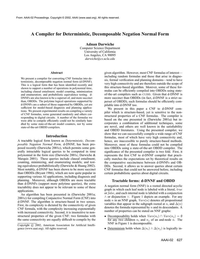
∧ or disjunction ∨. Figure 1 depicts an example. For any
node n in an NNF graph, Vars(n) denotes all propositional
variables that appear in the subgraph rooted at n, and ∆(n)
denotes the formula represented by n and its descendants. A
number of properties can be stated on NNF graphs:
• Decomposability holds when Vars(ni ) ∩ Vars(nj ) = ∅
for any two children ni and nj of an and-node n. The
NNF in Figure 1 is decomposable.
• Determinism holds when ∆(ni ) ∧ ∆(nj ) is logically in-
AAAI-02
627
CNF 2 DDNNF (n, Ω)
or
and
or
1.
2.
3.
4.
5.
6.
and
or
or
and and and and
or
if n is a leaf node, return clause2ddnnf(Clauses(n) | Ω)
ψ←cnf2key(Clauses(n) | Ω)
if cachen (ψ) 6= nil, return cachen (ψ)
Γ←case analysis(n, Ω)
cachen (ψ)←Γ
return Γ
and and and and
CASE ANALYSIS (n, Ω)
¬A
B
¬B
A
C
¬D
D
¬C
Figure 1: A negation normal form graph.
consistent for any two children ni and nj of an or-node n.
The NNF in Figure 1 is deterministic.
7. Σ←Sep(n, Ω)
8. if Σ = ∅, return CONJOIN(cnf2ddnnf(nl , Ω),cnf2ddnnf(nr , Ω))
9. X← choose a variable in Σ
10. WHILE CASE(X,true,Π):
11. if Π = ∅, α+ ←false
12. else α+ ←conjoin(Π, case analysis(n, Π ∪ Ω))
13. WHILE CASE(X,false,Π):
14. if Π = ∅, α− ←false
15. else α− ←conjoin(Π, case analysis(n, Π ∪ Ω))
16. return DISJOIN(α+ ,α− )
• Decision holds when the root node of the NNF graph is
a decision node. A decision node is a node labeled with
Figure 2: Compiling a CNF into d-DNNF.
or
and
and
true, false, or is an or-node having the form X α ¬X β ,
where X is a variable, α and β are decision nodes. Here,
X is called the decision variable of the node. The NNF
in Figure 1 does not satisfy the decision property since its
root is not a decision node.
• Ordering is defined only for NNFs that satisfy the decision
property. Ordering holds when decision variables appear
in the same order along any path from the root to any leaf.
Satisfiability and clausal entailment can be decided in linear time for decomposable negation normal form (DNNF)
(Darwiche 2001a). Moreover, its models can be enumerated
in output polynomial time, and any subset of its variables
can be forgotten (existentially quantified) in linear time. Deterministic, decomposable negation normal form (d-DNNF)
is even more tractable as we can count its models given
any variable instantiation in polytime (Darwiche 2001c;
Darwiche & Marquis 2001). Decision implies determinism. The subset of NNF that satisfies decomposability
and decision (hence, determinism) corresponds to Free Binary Decision Diagrams (FBDDs) (Gergov & Meinel 1994).
The subset of NNF that satisfies decomposability, decision (hence, determinism) and ordering corresponds to Ordered Binary Decision Diagrams (OBDDs) (Bryant 1986;
Darwiche & Marquis 2001). In OBDD notation, however,
or
and
the NNF fragment
and
X α ¬X β
> DNNF, where > stands for “less succinct than.”1 OBDDs are more tractable than DNNF, d-DNNF and FBDD.
General entailment among OBDDs can be decided in polytime. Hence, the equivalence of two OBDDs can be decided
in polytime. The equivalence of two DNNFs cannot be decided in polytime (unless P=NP). The equivalence question
is still open for d-DNNF and FBDD, although both support
polynomial probabilistic equivalence tests (Blum, Chandra,
& Wegman 1980; Darwiche & Huang 2002). For a comprehensive analysis of these forms, the reader is referred to
(Darwiche & Marquis 2001).
We close this section by noting that the polytime operations supported by DNNF are sufficient to implement
model-based diagnosers whose complexity is linear in the
size of compiled device, assuming the device is expressed as
a DNNF (Darwiche 2001a). Moreover, for planning and formal verification applications, there is no need for a polytime
test for general entailment as long as the goal (or property to
be verified) can be expressed as a CNF (clausal entailment
can be used here). Finally, polytime equivalence testing is
not needed here as it is only used to check for fixed points:
whether the models of some theory ∆t (reachable states at
time t) equal the models of some theory ∆t+1 (reachable
states at time t + 1), where ∆t |= ∆t+1 (the states reachable
at t are included in those reachable at t+1). The two theories
are equivalent in this case iff they have the same number of
models. Hence, counting models is sufficient to detect fixed
points in these applications.
is drawn more compactly as
Compiling CNF into d-DNNF
X
α
β . Hence, each non-leaf OBDD node generates three
NNF nodes and six NNF edges.
Immediate from the above definitions, we have the following strict subset inclusions OBDD ⊂ FBDD ⊂ d-DNNF
⊂ DNNF. Moreover, we have OBDD > FBDD > d-DNNF
628
AAAI-02
Figure 2 depicts the pseudocode of an algorithm for compiling a CNF into a d-DNNF. The presented algorithm uses a
1
That DNNF is strictly more succinct than d-DNNF assumes
the non-collapse of the polynomial heirarchy (Darwiche & Marquis
2001).
Figure 3: A decomposition tree for a CNF. Each leaf node is
labeled with a clause (a set of literals). Each internal node is
labeled with a separator (S) and a context (C).
data structure, known as a decomposition tree (dtree), which
is a full binary tree with its leaves corresponding to clauses
in the given CNF (Darwiche 2001a). Figure 3 shows an example dtree, where each leaf node is labeled with a clause
and each internal node is labeled with two sets of variables to be explained later. The algorithm works as follows. Each node n in the dtree corresponds to the set of
clauses, Clauses(n), appearing in the subtree rooted at n.
Let nl and nr denote the left and right children of node
n. If Clauses(nl ) and Clauses(nr ) do not share variables,
then we can convert Clauses(nl ) into a d-DNNF αl and
Clauses(nr ) into a d-DNNF αr and simply return αl ∧ αr
as the d-DNNF of Clauses(n). In general, Clauses(nl ) and
Clauses(nr ) do share variables, called a separator for dtree
node node n . In that case, we choose one of these variables,
call it X, and then perform a case analysis on it.
Case analysis. To perform case analysis on a variable X
is to consider two cases, one under which X is set to true and
another under which it is set to false. Under each case, X is
eliminated from the given set of clauses. If α+ is the result
of converting Clauses(n) into d-DNNF under X = true,
and if α− is the result of converting Clauses(n) into dDNNF under X = false, then (X ∧ α+ ) ∨ (¬X ∧ α− ) is a
d-DNNF equivalent to Clauses(n).2 Case analysis is implemented using the macro WHILE CASE(X,v,Π) on Lines 10
& 13, which replaces every occurrence of the variable X by
v, performs unit resolution, and then collects all derived literals (including X = v) in Π. Note here that Π not only
contains the literal X = v as suggested above, but also all
other literals derived by unit resolution (this leads to better
results in general). If unit resolution derives a contradiction,
Π is then the empty set.
2
This is known as the Shannon expansion of Clauses(n) in the
literature on Boolean logic. It was initially proposed by Boole,
however (Boole 1848).
Separators. We may have to perform case analysis on more than one variable before we can decompose
Clauses(nl ) and Clauses(nr ); that is, before we eliminate
every common variable between them. In general though,
we do not need to perform case analysis on every variable
common between Clauses(nl ) and Clauses(nr ). By setting
a variable X to some value, some clauses under nl or nr may
become subsumed, hence, eliminating some more variables
that are common between them. This is why the separator
for node n is defined with respect to a set of literals Ω on
Line 7. That is, Sep(n, Ω) is defined as the variables common between Clauses(nl ) | Ω and Clauses(nr ) | Ω, where
Clauses(.) | Ω is the result of conditioning the clauses . on
the literals Ω. That is, Clauses(.) | Ω is the set of clauses
which results from eliminating the variables in Ω from . and
replacing them by either true or false according to their signs
in Ω.3 Figure 3 depicts the separator for each node the given
dtree, assuming Ω = ∅.
The choice of which variable to set next from the separator Sep(n, Ω) on Line 9 has an effect on the overall time
to compile into d-DNNF and also on the size of resulting dDNNF. In our current implementation, we choose the variable that appears in the largest number of binary clauses.
Finally, the base case in the recursive procedure of Figure 2
is when we reach a leaf node n in the dtree (Line 1), which
means that Clauses(n) contains a single clause. In this case,
clause2ddnnf(.) is a constant time procedure which converts a clause into a d-DNNF.4
Unique nodes. Another technique we employ comes
from the literature on OBDDs and is aimed at avoiding the
construction of redundant NNF nodes. Two nodes are redundant if they share the same label (disjunction or conjunction)
and have the same children. To avoid redundancy, we cache
every constructed NNF node, indexed by its children and label. Before we construct a new NNF node, we first check
the cache and construct the node only if no equivalent node
is found in the cache. This technique is implicit in the implementation of CONJOIN and DISJOIN.5
Caching. Probably the most important technique we employ comes from the literature on dynamic programming.
Specifically, each time we compile Clauses(n) | Ω into a
d-DNNF α, we store (the root of) d-DNNF α in a cache associated with dtree node n; see Line 5. When the algorithm
tries to compile Clauses(n) | Ω again, the cache associated with node node n is first checked (Lines 2&3). The
cache key we use to store the d-DNNF α is a string generated from Clauses(n) | Ω: each non-subsumed clause in
Clauses(n) | Ω has two characters, one capturing its identity and the other capturing its literals. The generation of
such a key is expensive, but the savings introduced by this
3
This process is also known as restriction in the literature on
Boolean logic.
4
AW
clause lV
1 , . . . , lm can be converted into a d-DNNF as folm
i−1
lows: i=1 li j=1 ¬lj .
5
CONJOIN and DISJOIN will construct nodes with multiple children when possible. For example, when conjoining two conjunctions, CONJOIN will generate one node labeled with ∧ and have it
point to the children of nodes being conjoined.
AAAI-02
629
caching scheme are critical. This caching scheme is a major improvement on the one proposed in (Darwiche 2001a;
2001c). In the cited work, a context for node n, Context(n),
is defined as the set of variables that appear in the separator of some ancestor of n and also in the subtree rooted
at n; see Figure 3. It is then suggested that d-DNNF α
of Clauses(n) | Ω be cached under a key, which corresponds to the subset of literals Ω pertaining to the variables
in Context(n). That is, if Clauses(n) = {A ∨ ¬B, C ∨ D},
then Clauses(n) | {A} could be cached under key A, and
Clauses(n) | {¬B} could be cached under key ¬B, hence,
generating two different subproblems. Using our caching
approach, both Clauses(n) | {A} and Clauses(n) | {¬B}
will generate the same key, and will be treated as instances of
the same subproblem, since both are equivalent to {C ∨ D}.
Constructing dtrees. Another major factor that affects
the behavior of our algorithm is the choice of a dtree. At
first, one may think that we need to choose a dtree where
the sizes of separators are minimized. As it turns out, however, this is only one important factor which needs to be balanced by minimizing the size of contexts as defined above.
The smaller the separators, the fewer case analyses we have
to consider. The smaller the contexts, the higher the cache
hit rate. Unfortunately, these two objectives are conflicting:
dtrees with small separator tend to have large contexts and
the other way around. A better paramater to optimize is the
size of clusters. The cluster of node n is the union of its
separator and context. The size of the maximum cluster -1
is known as the dtree width (Darwiche 2001a). In our current implementation, we construct dtrees using the method
described in (Darwiche & Hopkins 2001), which is based on
recursive hypergraph decomposition. Specifically, the given
CNF ∆ is converted into a hypergraph G, where each clause
in ∆ is represented as a hypernode in G. Each variable X
in CNF ∆ is then represented as a hyperedge in G, which
connects all hypernodes (clauses) of G in which X appears.
Once the hypergraph G is constructed, we partition it into
two pieces Gl and Gr , hence, partitioning the set of clauses
in ∆ into two corresponding sets ∆l and ∆r . This decomposition corresponds to the root of our dtree, and the process can be repeated recursively until the set of clauses in
∆ are decomposed into singletons. Hypergraph decomposition algorithms try to attain two objectives: minimize the
number of hyperedges that cross between Gl and Gr , and
balance the sizes of Gl and Gr . These two objectives lead
to generating dtrees with small widths as has been shown in
(Darwiche & Hopkins 2001). The construction of a dtree according to the above method is quite fast and predictable, so
we don’t include the time for converting a CNF into a dtree
in the experimental results to follow. We have to mention
two facts though about the method described above. First,
the hypergraph partitioning algorithm we use is randomized,
hence, it is hard to generate the same dtree again for a given
CNF. This also means that there is no guarantee that one
would obtain the same d-DNNF for a given CNF, unless the
same dtree is used across different runs. Second, the hypergraph partitioning algorithm requires a balance factor, which
is used to enforce the balance constraint. We have found that
a balance factor of 3/1 seems to generate good results in gen-
630
AAAI-02
eral. Therefore, if one does not have time to search across
different balance factors, a balance factor of 3/1 is our recommended setting.
We close this section by noting that to compile a CNF ∆
into a d-DNNF, we have to first construct a dtree with root n
for ∆ and then call cnf2ddnnf(n, ∅).
Experimental results
We will now apply the presented CNF 2 DDNNF compiler to
a number of CNFs. The experiment were run on a Windows
platform, with a 1GHz processor. Our implementation is
in LISP! We expect a C implementation to be an order of
magnitude faster. The compiler is available through a web
interface—please contact the author for details.
Random CNF formulas
Our first set of CNFs comes from SATLIB6 and includes satisfiable, random 3CNF formulas in the crossover region, in
addition to formulas corresponding to graph coloring problems; see Table 1.7 Random 3CNF formulas (uf50–uf200)
could be easily compiled with less than a minute on average for the largest ones (200 vars). Compiling such CNFs
into OBDDs using the state-of-the-art CUDD8 compiler was
not feasible in general.9 For example, we could not compile the first instance of uf100 within four hours. Moreover,
the first instance in uf50 takes about 20 minutes to compile.
More than 2 million nodes are constructed in the process,
with more than 500 thousand nodes present in memory at
some point (the final OBDD has only 82 nodes though). We
have to point out here that we used CUDD in a straightforward manner. That is, we simply constructed an OBDD
for each clause and then conjoined these clauses according to their order in the CNF. There are more sophisticated
approaches for converting CNFs into OBDDs that have
been reported recently (Aloul, Markov, & Sakallah 2001;
December 2001). No experimental results are available at
this stage, however, on compiling random CNFs into OBDDs using these approaches. We will report on these approaches with respect to other datasets later on though.
We also report on the compilation of graph coloring problems in Table 1 (flat100 and flat200). As is clear from the table, these CNFs can be easily compiled into small d-DNNFs
that have a large number of models. Each one of these models is a graph coloring solution. Not only can we count these
solutions, but we can also answer a variety of queries about
these solutions in linear time. Examples: How many solutions set the color of node n to c? Is it true that when
node n1 is assigned color c1 , then node n2 must be assigned
color c2 ? And so on? Although compiling a flat200 CNF
takes 11 minutes on average, answering any of the previous
queries can be done by simply traversing the compiled dDNNF only once (Darwiche 2001c), which takes less than a
6
http://www.intellektik.informatik.tu-darmstadt.de/SATLIB/
Sets uf50 and uf100 contain 1000 instances each. We only use
the first 100 instances.
8
http://vlsi.colorado.edu/ fabio/CUDD/
9
We used the sift-converge dynamic ordering heuristic in our
experiments.
7
Name
Vars/Clause
uf50
uf100
uf150
uf200
flat100
flat200
50/218
100/430
150/645
200/860
300/1117
600/2237
d-DNNF
nodes
111
1333.3
3799.8
4761.8
1347.2
4794.9
d-DNNF
edges
258.4
4765.3
15018.5
19273.3
8565.2
46951.3
Model
count
362.2
1590706.1
68403010
1567696500
8936035
2.2202334e+13
Time
(sec)
1
2
8
37
4
636
Table 1: CNF benchmarks from SATLIB. Each set contains a 100 instances. We report the average over all instances.
700000
600000
Nodes#
Edges#
Time (ms)
Boolean Circuits
500000
400000
300000
200000
100000
0
0.5 0.6 0.7 0.8 0.9 1.0 1.1 1.2 1.3 1.4 1.5 1.6 1.7 1.8 1.9 2.0 2.1 2.2 2.3 2.4 2.5 2.6 2.7 2.8 2.9 3.0 3.1 3.2 3.3 3.4 3.5
Figure 4: Difficulty of compilation according to clauses/vars
ratio. Each point is the average over 100 instances.
second in this case. Hence, the compilation time is amortized over all queries which makes the time-to-compile a
worthy investment in this case. We note here that the first
instance of flat100 could not be compiled into an OBDD using CUDD within a cutoff time of 1 hour. One can count the
models of flat100 efficiently however using the RELSAT10
model counter, but we report in the following section on
other CNFs which could not be handled efficiently using
RELSAT.
We also experimented with planning CNFs from SATLIB.
We could compile blocks-world CNFs anomaly, medium,
huge, and large.a within a few minutes each. But we could
not compile large.b, nor the logistics CNFs within a few
hours.
We close this section by noting that random 3CNF formulas in the crossover region, those with clauses/vars ratio
of about 4.3, are easier to compile than formulas with lower
ratios. The same has been observed for counting models,
where the greatest difficulty is reported for ratios around 1.2
by (Birnbaum & Lozinskii 1999) and around 1.5 by (Ba10
yardo & Pehoushek 2000). Figure 4 plots information about
compilations of random 3CNFs with 50 variables each, for
clauses/vars ratio ranging from .5 to 3.5 at increments of .1.
As is clear from this plot, the peak for the number of nodes,
number of edges, and time is around a ratio of 1.8.
http://www.almaden.ibm.com/cs/people/bayardo/vinci/index.html
We now consider CNFs which correspond to digital circuits.
Suppose we have a circuit with inputs I, outputs O and let
W stand for all wires in the circuit that are neither inputs
nor outputs. We will distinguish between three types of representations for the circuit:
Type I representation: A theory ∆ over variables I, O, W
where the models of ∆ correspond to instantiations of
I, O, W that are compatible with circuit behavior. A CNF
corresponding to Type I representation can be easily constructed and in a modular way by generating a set of clauses
for each gate in the circuit.11
Type II representation: A theory ∆ over input/output
variables I, O, where the models of ∆ correspond to input/output vectors compatible with circuit behavior. If
∆ is a Type I representation, then ∃W ∆ is a Type II
representation.12
Type III representation for circuit output o: A theory over
inputs I, where the models correspond to input vectors that
generate a 1 at output o. If ∆ is a Type II representation,
then ∃o.∆ ∧ o is a Type III representation for output o.
Clearly, Type I is more expressive than Type II, which
is more expressive than Type III. The reason we draw this
distinction is to clarify that in the formal verification literature, one usually constructs Type III representations for circuits since this is all one needs to check the equivalence of
two circuits. In AI applications, however, such as diagnosis,
one is mostly interested in Type I representations, which are
much harder to obtain.
We compute Type II representations by simply replacing
Lines 12 & 15 in CNF 2 DDNNF by
α+ ←conjoin(Π0 , case analysis(n, Π ∪ Ω)),
11
Type I representations are called Circuit Consistency Functions in (Aloul, Markov, & Sakallah 2001; December 2001).
12
Recall: ∃w∆, where w is a single variable, is defined as ∆+ ∨
∆− , where ∆+ (∆− ) is the result of replacing w with true (false)
in ∆. ∃W ∆ is the result of quantifying over variables in W , one
at a time (Darwiche & Marquis 2001).
AAAI-02
631
and
−
α ←conjoin(Π , case analysis(n, Π ∪ Ω)),
respectively, where Π0 is obtained from Π by removing all literals corresponding to variables in W . We
also have to modify the boundary condition handled by
CLAUSE 2 DDNNF , so that CLAUSE 2 DDNNF (.) returns true
if the clause . contains a literal pertaining to W , and behaves
as usual otherwise. Given the above changes—which implement the proposal given in (Darwiche 2001a) for existential
quantification—cnf2ddnnf(n, ∅) is then guaranteed to return ∃W ∆ in d-DNNF, where n is the root of a dtree for
CNF ∆.13
To compute efficient Type III representations, one needs
to use multi-rooted NNFs, where each root corresponds to
the compilation of one circuit output. This is how it is done
in the formal verification literature, where multi-rooted OBDDs are known as shared OBDDs. Our compiler does not
handle multi-rooted d-DNNFs yet, so we do not report on
Type III representations.
Tables 2 and 3 contain results on the first five circuits in
the ISCAS85 benchmark circuits.14 We were able to obtain
Type I and Type II representations for all these circuits expressed as d-DNNFs. The most difficult was c1908, which
took around 1.5 hrs, followed by c880 which took around
30 minutes. We are not aware of any other compilations of
these circuits of Types I and II, although the formal verification literature contains successful compilations of Type
III, represented as multi-rooted OBDDs. We could not compile c499, c880, c1355, nor c1908 into Type I OBDDs using CUDD, nor could we count their models using RELSAT,
within cutoff times of 1hr, 1hr, 1hr and 3hrs, respectively
(we actually tried CUDD on c499 for more than a day). For
c432, we tried several OBDD ordering heuristics. The best
OBDD we could obtain for this circuit had 15811 nodes.
We note here that although d-DNNF does not support
a deterministic test of equivalence, one can easily test the
equivalence of a d-DNNF ∆, and a CNF Γ = γ1 ∧ . . . ∧ γm ,
which corresponds to a Type I representation of a circuit. By
construction, the number of models for Γ is 2k , where k is
the number of primary inputs for the circuit. Therefore, ∆
and Γ are equivalent iff (1) the number of models for ∆ is 2k
and (2) ∆ |= Γ. The first condition can be checked in time
linear in the size of ∆ since d-DNNF supports model counting in linear time. The second condition can be checked
by verifying that ∆ |= γi for each i, a test which can also
be performed in time linear in the size of ∆ since d-DNNF
supports a linear test for clausal entailment. We actually use
the above technique for checking the correctness of our dDNNF compilations.
Table 4 contains further results from ISCAS89.15 These
are sequential circuits, which have been converted into com13
In general, this only guarantees that the result is in DNNF
(Darwiche 2001a). For CNFs corresponding to digital circuits,
however, determinism is also guaranteed due to the following property: for every instantiation α of I, O, there is a unique instantiation β of W such that ∆ ∧ α |= β.
14
http://www.cbl.ncsu.edu/www/CBL Docs/iscas85.html
15
http://www.cbl.ncsu.edu/www/CBL Docs/iscas89.html
632
AAAI-02
Name
Vars/Clause
c432
c499
c880
c1355
c1908
196/514
243/714
443/1112
587/1610
913/2378
0
d-DNNF
nodes
2899
691803
3975728
338959
6183489
d-DNNF
edges
19779
2919960
7949684
3295293
12363322
Clique
size
28
23
24
23
45
Time
(sec)
6
448
1893
809
5712
Table 2: Type I compilations of ISCAS85 circuits.
Name
I/O vars
c432
c499
c880
c1355
c1908
36/7
41/32
60/26
41/32
33/25
d-DNNF
nodes
952
68243
718856
65017
326166
d-DNNF
edges
3993
214712
2456827
201576
1490315
Time
(sec)
1
127
1774
483
4653
Table 3: Type II compilations of ISCAS85 circuits.
binational circuits by cutting feedback loops into flip-flops,
treating a flip-flop’s input as a circuit output and its output
as a circuit input. Most of these circuits are easy to compile and have relatively small d-DNNFs. Type I OBDD
representations for some ISCAS89 circuits are reported in
(Aloul, Markov, & Sakallah 2001; December 2001), which
is probably the most sophisticated approach for converting CNFs into OBDDs. In addition to proposing a new
method for ordering OBDD variables based on the connectivity of given CNF, a proposal is made for ordering the
clauses during the OBDD construction process. (Aloul,
Markov, & Sakallah 2001; December 2001) report on the
maximum number of OBDD nodes during the construction process, not on the size of final OBDDs constructed.
Yet, their experiments appear to confirm the theoretical results reported in (Darwiche & Marquis 2001) on the relative succinctness of d-DNNF and OBDD representations.
For example, circuits s832, s953, s1196 and s1238 were
among the more difficult ones in these experiments, leading to constructing 115 × 103 , 1.8 × 106 , 2 × 106 , and
2×106 nodes, respectively—s1238 is the largest circuit they
report on. These numbers are orders of magnitude larger
than what we report in Table 4.16 We note here that the
total number of nodes constructed by our d-DNNF compiler is rarely more than twice the number of nodes in the
final d-DNNF.17 We finally note that no experimental results are provided in (Aloul, Markov, & Sakallah 2001;
16
One has to admit though that it is hard to tell exactly how much
of this difference is due to relative succinctness of OBDD vs dDNNF, and how much of it is due to the effectiveness of different
compilation techniques, since none of the compilers discussed are
guaranteed to generate optimal OBDDs or d-DNNFs.
17
This is in contrast to OBDD compilers, where the number of
intermediate OBDD nodes can be much larger than the size of final
OBDD returned. We believe this is due to the top-down construction method used by our compiler, as opposed to the bottom-up
methods traditionally used by OBDD compilers.
Name
Vars/Clause
s298
s344
s349
s382
s386
s400
s444
s499
s510
s526
s526n
s635
s641
s713
s820
s832
s938
s953
s967
s991
s1196
s1238
s1423
s1488
s1494
s1512
s3330
s3384
136/363
184/429
185/434
182/464
172/506
186/482
205/533
175/491
236/635
217/638
218/639
320/762
433/918
447/984
312/1046
310/1056
512/1233
440/1138
439/1157
603/1337
561/1538
540/1549
748/1821
667/2040
661/2040
866/2044
1961/4605
1911/4440
d-DNNF
nodes
830
962
1017
1034
1401
1021
1091
1090
967
2621
2611
1360
7062
7128
2774
2757
2207
11542
20645
2382
12554
14512
112701
6338
6827
12560
358093
44487
d-DNNF
edges
4657
4973
5374
5081
10130
5137
5872
5565
5755
19605
20115
4845
84596
90901
21365
21224
12342
110266
443233
13107
261402
288143
1132322
62175
64888
140384
8889410
392223
Clique
size
12
9
10
17
21
18
16
20
38
22
22
9
21
21
29
28
14
64
60
8
51
53
24
49
51
21
43
17
Time
(sec)
1
1
1
1
2
1
1
2
2
1
1
1
1
10
2
2
2
14
117
2
60
58
162
11
12
27
5853
45
Table 4: Type I compilations of ISCAS89 circuits.
December 2001) for Type I OBDD representations of ISCAS85 circuits, which are much harder to compile than ISCAS89 circuits.
One implication of our ability to compile these circuits is
that we can now perform a variety of reasoning tasks about
these circuits in time linear in the size of given d-DNNF.
Some example queries: Given a distribution over the circuit
inputs, what is the probability that Wire 45 is high? How
may circuit inputs will generate a high on the first circuit
output and a low on the fifth output? Is it true that whenever
Wires 33 and 87 are high, then Wire 19 must be low? How
may input vectors will generate a particular output vector?
Each one of these queries can be answered by a single traversal of the d-DNNF circuit representation (Darwiche 2001b;
2001a; 2001c).
We also report in Tables 2–4 on the best clique sizes obtained for these circuits when converting their structures into
jointrees (Jensen, Lauritzen, & Olesen 1990). This is needed
for reasoning about these circuits probabilistically using
state-of-the-art algorithms for Bayesian networks. These
algorithms have exponential complexity in the clique size.
Hence, most of these circuits are outside the scope of such
algorithms. We are not aware of any algorithm for probabilistic reasoning which can handle these circuits, except
the one we report on in (Darwiche 2001b) which is based
on these d-DNNF compilations. We close this section
by noting that the algorithm reported in (Darwiche 2001a;
2001c) also has a time complexity which is exponential in
the clique size. Hence, most of the CNFs we considered in
this paper are outside the scope of the mentioned algorithm.
Relationship to Davis-Putnam
One cannot but observe the similarity between our proposed
algorithm and the Davis-Putnam (DP) algorithm for propositional satisfiability (Davis, Logemann, & Loveland 1962),
and its recent extensions for counting propositional models:
the CDP algorithm in (Birnbaum & Lozinskii 1999) and the
DDP algorithm in (Bayardo & Pehoushek 2000).
The DP algorithm solves propositional satisfiability by
performing case analysis until a solution is found or an inconsistency is established. When performing case analysis on variable X, the second value for X is considered
only if the first value does not lead to a solution. The
CDP algorithm in (Birnbaum & Lozinskii 1999) observed
that by always considering both values, we can extend the
DP algorithm to count models since ModelCount(∆) =
ModelCount(∆+ ) + ModelCount(∆− ), where ∆+ and
∆− are the result of setting X to true and to false, respectively, in ∆. The DDP algorithm in (Bayardo & Pehoushek 2000) incorporated yet another idea: If ∆ can be
decomposed into two disconnected subsets ∆1 and ∆2 , then
ModelCount(∆) = ModelCount(∆1 )ModelCount(∆2 ).
Hence, DDP will apply case analysis until the CNF is disconnected into pieces, in which case each piece is attempted
independently.
The CDP algorithm can in fact be easily adapted to compile a CNF into a d-DNNF, by simply constructing the NNF
fragment X ∧ cdp(∆+ ) ∨ ¬X ∧ cdp(∆− ) each time a case
analysis is performed on variable X. Here, cdp(.) is the result of compiling . into d-DNNF using the same algorithm
recursively. This extension of CDP will generate a strict
subset of d-DNNF: the one which satisfies the decision and
decomposability properties (hence, an FBDD) and that also
has a tree structure (FBDDs have a graph structure in general). FBDDs are known to be less succinct than d-DNNFs,
even in their graph form (Darwiche & Marquis 2001). The
tree-structured form is even more restrictive.
The DDP algorithm can also be easily adapted to compile a CNF into a d-DNNF, by constructing the NNF fragment X ∧ ddp(∆+ ) ∨ ¬X ∧ ddp(∆− ) each time a case
analysis is performed on X, and by constructing the fragment ddp(∆1 ) ∧ ddp(∆2 ) each time a decomposition is
performed as given above. This extension of DDP will actually generate d-DNNFs which are not FBDDs, yet are still
tree-structured which is a major limitation. The important
point to stress here is that any CNF which can be processed
successfully using the DDP algorithm, can also be compiled
successfully into a d-DNNF.
The algorithm we present can be viewed as a further generalization of the discussed DDP extension in the sense that it
generates graph NNFs as opposed to tree NNFs. The graph
structure is due to two features of CNF 2 DDNNF: the caching
and unique-node schemes. Each time a node is looked up
from a cache, its number of parents will potentially increase
by one. Moreover, the CONJOIN and DISJOIN operations
AAAI-02
633
will often return a pointer to an existing NNF node instead
of constructing a new one, again, increasing the number of
parents per node.18 Another major difference with the above
proposed extension of DDP is the use of dtrees to guide the
decomposition process as they restrict the set of variables
considered for case analysis at any given time. The use of
dtrees can then be viewed as a variable splitting heuristic
which is geared towards decomposition as opposed to solution finding.
Conclusion
We presented a compiler for converting CNF formulas
into deterministic, decomposable negation normal form (dDNNF). This is a logical form that has been identified recently and shown to support a number of operations in polynomial time, including clausal entailment; model counting, minimization and enumeration; and probabilistic equivalence testing. d-DNNFs are also known to be a superset of, and more succinct than, OBDDs. The logical operations supported by d-DNNFs are a subset of those supported by OBDDs, yet are sufficient for model-based diagnosis and planning applications. We presented experimental results on compiling a variety of CNF formulas, some
generated randomly and others corresponding to digital circuits. A number of the formulas we were able to compile
efficiently could not be similarly handled by some state-ofthe-art model counters, nor by some state-of-the-art OBDD
compilers. Moreover, our ability to successfully compile
some of these CNFs allowed us to answer some queries for
the very first time.
Acknowledgments
The author would like to thank Fadi Aloul, Roberto Bayardo, Rolf Haenni and Pierre Marquis for helpful comments and suggestions regarding earlier drafts of this paper.
This work has been partially supported by NSF grant IIS9988543 and MURI grant N00014-00-1-0617.
References
Aloul, F. A.; Markov, I. L.; and Sakallah, K. A. 2001.
Faster SAT and smaller BDDs via common function structure. In International Conference on Computer Aided Design (ICCAD), 443–448.
Aloul, F. A.; Markov, I. L.; and Sakallah, K. A. December,
2001. Faster SAT and smaller BDDs via common function
structure. Technical Report CSE-TR-445-01, Computer
Science and Engineering Division, University of Michigan.
Bayardo, R., and Pehoushek, J. 2000. Counting models
using connected components. In AAAI, 157–162.
Birnbaum, E., and Lozinskii, E. 1999. The good old DavisPutnam procedure helps counting models. Journal of Artificial Intelligence Research 10:457–477.
18
(Bayardo & Pehoushek 2000) rightfully suggest that “learning
goods,” which corresponds to caching non-zero counts, is essential
for efficient counting of models, but do not pursue the technique
citing technical difficulties.
634
AAAI-02
Blum, M.; Chandra, A. K.; and Wegman, M. N. 1980.
Equivalence of free Boolean graphs can be decided probabilistically in polynomial time. Information Processing
Letters 10(2):80–82.
Boole, G. 1848. The calculus of logic. The Cambridge and
Dublin Mathematical Journal 3:183–198.
Bryant, R. E. 1986. Graph-based algorithms for Boolean
function manipulation. IEEE Transactions on Computers
C-35:677–691.
Darwiche, A., and Hopkins, M. 2001. Using recursive decomposition to construct elimination orders, jointrees and
dtrees. In Trends in Artificial Intelligence, Lecture notes in
AI, 2143. Springer-Verlag. 180–191.
Darwiche, A., and Huang, J. 2002. Testing equivalence
probabilistically. Technical Report D–123, Computer Science Department, UCLA, Los Angeles, Ca 90095.
Darwiche, A., and Marquis, P. 2001. A perspective on
knowledge compilation. In Proc. International Joint Conference on Artificial Intelligence (IJCAI), 175–182.
Darwiche, A. 2001a. Decomposable negation normal form.
Journal of the ACM 48(4):1–42.
Darwiche, A. 2001b. A logical approach to factoring belief networks. Technical Report D–121, Computer Science
Department, UCLA, Los Angeles, Ca 90095. To appear in
KR-02.
Darwiche, A. 2001c. On the tractability of counting theory
models and its application to belief revision and truth maintenance. Journal of Applied Non-Classical Logics 11(12):11–34.
Davis, M.; Logemann, G.; and Loveland, D. 1962. A
machine program for theorem proving. CACM 5:394–397.
Gergov, J., and Meinel, C. 1994. Efficient analysis and
manipulation of OBDDs can be extended to FBDDs. IEEE
Transactions on Computers 43(10):1197–1209.
Jensen, F. V.; Lauritzen, S.; and Olesen, K. 1990. Bayesian
updating in recursive graphical models by local computation. Computational Statistics Quarterly 4:269–282.