From: AAAI-98 Proceedings. Copyright © 1998, AAAI (www.aaai.org). All rights reserved.
Learning Evaluation
Justin
Functions for Global Optimization
Boolean Satisfiability
and
A. Boyan and Andrew W. Moore
Computer Science Department
Carnegie Mellon University
Pittsburgh, PA 15213
(jab,awm}@cs.cmu.edu
Abstract
This paper describes STAGE, a learning approach
to automatically improving search performance
on optimization problems. STAGE
learns an evaluation function which predicts the outcome of
a local search algorithm, such as hillclimbing or
WALKSAT, as a function of state features along
its search trajectories. The learned evaluation
function is used to bias future search trajectories toward better optima. Wepresent positive
results on six large-scale optimization domains.
Introduction
VLSI design, engineering design, Boolean formula satisfaction, bin-packing, medical treatment planning and
Bayes net structure finding are all examples of global
optimization--the problem of finding the best possible configuration from a large space of possible configurations. Formally, a global optimization problem
consists of a state space X and an objective function
Obj : X --+ ~. The goal is to find astate x* E X
which minimizes Obj. If X is large, then finding x*
is generally intractable unless the problem has a very
specialized structure (e.g., a linear program). However,
many general-purpose local search algorithms attempt
to exploit Obj’s structure to locate good approximate
optima; for example, hillclimbing, simulated annealing, and tabu search. All of these work by imposing
a neighborhood relation on the states of X and then
searching the graph that results, guided by Obj.
Local search has been likened to "trying to find the
top of Mount Everest in a thick fog while suffering
from amnesia" (Russell 8~ Norvig 1995, pall). The
climber considers each step by consulting an altimeter
and deciding whether to take the step based on the
change in altitude. But suppose the climber has access
to not only an altimeter, but also additional senses and
instruments--for example, the current x and y location, the slope of the ground underfoot, and whether or
Copyright (~)1998, AmericanAssociation for Artificial
Intelligence (www.aaai.org).All rights reserved.
not the current location is on a trail. These additional
"features" may enable the climber to make a more
informed, more foresightful, evaluation of whether to
take a step.
In real optimization domains, such additional state
features are generally plentiful. Practitioners of local search algorithms often append additional terms to
their objective function, and then spend considerable
effort tweaking the coefficients. This excerpt, from a
book on VLSI layout by simulated annealing (Wong,
Leong, &Liu 1988), is typical:
Clearly, the objective function to be minimized
is the channel width w. However, w is too crude a
measure of the quality of intermediate solutions.
Instead, for any valid partition, the following cost
function is used:
C = w~ + Ap .p2 + Au ¯ g
(1)
U measures the sparsity of the horizontal tracks, while
p measures the longest path length in the current partition. In this application, the authors hand-tuned the
coefficients of the extra state features p2 and U, setting
Ap = 0.5 and )~v -- 10. (We will show that our algorithm learned to assign, counterintuitively, a negative
value to )~v, and achieved much better performance.)
Similar examples of evaluation functions being manually configured and tuned for good performance can
be found in, e.g., (Falkenauer ~ Delchambre 1992;
Szykman ~ Cagan 1995).
The question we address is the following: can extra features of an optimization problem be incorporated automatically into improved evaluation functions, thereby guiding search to better solutions?
The STAGE Algorithm
STAGE analyzes sample trajectories
and automatically
constructs predictive evaluation functions. It then
uses these new evaluation functions to guide further
search. A preliminary version of STAGE, described in
(Boyan & Moore 1997), showed promising performance
on VLSIlayout. This paper describes an improved version of STAGE
with superior results on VLSIlayout and
thorough results for five other global optimization domains. Wealso overview the theoretical foundations
of STAGE, one consequence of which is an extension allowing STAGE tO accelerate non-monotonic search procedures such as WALKSAT.
Learning to Predict
The performance of a local search algorithm depends
on the state from which the search starts.
Wecan
express this dependence in a mapping from starting
states x to expected search result:
Y~(z) =defexpected best Obj value seen on a tra- (2)
jectory that starts from state z and
follows local search methodlr
Here, ~r represents a local search methodsuch as hillclimbing or simulated annealing. V~ (x) evaluates x’s
promise as a starting state for 7r.
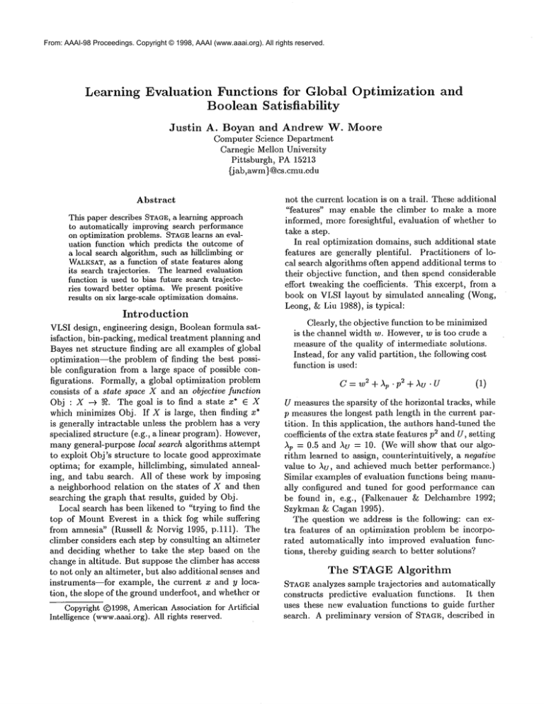
For example, consider
minimizing the onedimensional function Obj (z) = (Ixl - 10) cos(2rx)
the domain X = [-10, 10], as depicted in Figure 1.
Assuming a neighborhood structure on this domain
where tiny moves to the left or right are allowed,
hillclimbing (greedy descent) search clearly leads
a suboptimal local minimumfor all but the luckiest
of starting points. However, the quality of the local
minimumreached does correlate strongly with the
starting position: V’r(x) ~ I - 10. Ga thering da ta
from only a few suboptimal trajectories,
a function
approximator can easily learn to predict that starting
near z = 0 will lead to good performance.
-’o
vvvvvvv
,llvvvv
io
,
Training data for supervised learning of V~ may be
readily obtained by running ~r from different starting points. Moreover, if the algorithm r behaves as
a Markov chain--i.e.,
the probability of moving from
state x to z’ is the same no matter when z is visited
and what states were visited previously--then intermediate states of each simulated trajectory may also be
considered alternate "starting points" for that search,
and thus used as training data for V~as well. This insight enables us to get not one but perhaps hundreds of
pieces of training data from each trajectory sampled.
For the remainder of this paper, except in the section
on WALKSAT,
we will set zr to be stochastic hillclimbing, rejecting equi-cost moves, terminating as soon as
a fixed number (patience) of consecutive moves produces no improvement. This choice of ~r satisfies the
Markovproperty. Wewill also always use simple linear
or quadratic regression to fit V~, since training these
models incrementally is extremely efficient in time and
memory (Boyan 1998).
Using
Weapproximate V~ using a function approximation
model such as polynomial regression, where states x
are encoded as real-valued feature vectors. As discussed above, these input features may encode any
relevant properties of the state, including the original
objective function Obj(x) itself. Wedenote the mapping from states to features by F : X --+ ~D, and our
approximation of V’~ (z) by V~ (F(z)).
Predictions
The learned evaluation function ~Z~(F(x)) evaluates
how promising x is as a starting point for algorithm~.
~
To find the best starting point, we must optimize V
over X. Wedo this by applying stochastic hillclimbing
with V~ instead of Obj as the evaluation function)
.........................
produces
newira.i~ing data
Run ~ to
optimize
Obj/ for q~; retrainthe fitte?-.
2
produces
goodnew
starting
state.[or..~
.......
.o
Figure 1: Left: Obj (z) for a one-dimensional minimization domain. Right: the value function V~(z) which
predicts hillclimbing’s performance on that domain.
the
Hillclimbto
optimize V~
Figure 2: A diagram of the main loop of STAGE
The STAGEalgorithm_provides
a framework for
learning and exploiting V~ on a single optimization
instance. As illustrated in Figure 2, STAGE
repeatedly
alternates betweentwo different stages of local search:
running the original method ~r on Obj, and running
hillclimbing on V~ to find a promising new starting
state for ~r. Thus, STAGE can be viewed as a smart
multi-restart approach to local search.
1Note that even if V" is smooth with respect
to the
feature space--as it surely will be if we represent V~ with a
simple model like quadratic regression--it
may still give rise
to a complex cost surface with respect to the neighborhood
structure
on X. The existence
of a state
with a set of
features similar to the current state’s does not imply there
is a step in state-space that will take us to that state.
STAGEeffectively plots a single long trajectory
through the state space, periodically switching between the original objective function Obj(x) and the
newly-learned evaluation function 1) ~ (x). The trajectory is only broken if the l) ~r search phase accepts no
moves, indicating that x is a local minimumof both
evaluation functions. Whenthis occurs, STAGE resets
the search to a random starting state.
0J2
0.08
0.06
(4a)
0.04
0.02
0
Illustrative
30
Example
Wewill now work through a detailed illustrative example of STAGE
in operation. Then we will provide results
on six large, difficult, global optimization problems.
Our example comes from the practical, NP-complete
domain of bin-packing (Coffman, Garey, ~ Johnson
1996). In bin-packing, we are given a bin capacity C
and a list L = (al, a2, ...an) of n items, each having a
size s(ai) > 0. The goal is to pack the items into as
few bins as possible. Figure 3 depicts an example binpacking instance with thirty items. Packed optimally,
these items fill 9 bins exactly to capacity.
HCon Obj
0.1
25
20
t5
Feature
#t: Obj(x)nu
mber bin
ofs use
d
10
VpLO
(first iteration)-15
’i
(4b)
0.1
Va
0.12
HC on Obj
HC on Obj
0.1
"6 0.08
0.o6
(4c)
0.04
~m
0.02
0
i
30
=
i
i
25
20
15
10
Feature#1: Obj(x) = number
of bins used
Vpi_l (second iteration)
8 ......
9---~
lo
2o
r
11Sl-
Figure 3: A small example bin-packing instance
To apply local search, we define a neighborhood operator which moves a single random item to a randomnew bin having sufficient spare capacity. STAGE
predicts the outcome of stochastic hillclimbing using
quadratic regression over two features of the state x:
(4d)
~(x)
1. The actual objective function, Obj = ~ of bins used.
2. Var = the variance in fullness of the non-emptybins.
This feature is similar to a cost function term introduced in (Falkenauer & Delchambre 1992).
Figure 4 depicts the first three iterations of a STAGE
run on the example instance. On the first iteration (4a), STAGE
hillclimbs from the starting state
(Obj = 30, Var = 0.011) to a local optimum (Obj
13, Var = 0.019). Training each of the 18 states of that
trajectory to predict the outcome13 results in the flat
l) ~ ~
function shownin 4b. Hillclimbing on this flat l)
accepts no moves, so STAGE
resets to the initial state.
11:22:
~
15
""
0.12
HCon Obj
HCon Obj
on VpL1
0.1 ¯ HC
HCon Obj
J~
"6 0.08
0.06
(4e)
:~ 0.04
~2
0.02
0
Figure 4:
30
25
20
15
tO
Feature#1: Obj(x) = numberof Nasused
STAGE working
on the bin-packing example
On the second iteration
of STAGE(4c), the new
stochastic hillclimbing trajectory happens to do better than the first, finishing at a local optimum(Obj
11, Var = 0.022). Our training set is augmented with
target values of 11 for all states on the new trajectory. The resulting quadratic V~ already has significant structure (4d). Note how the contour lines
V~, shownon the base of the surface plot, correspond
to smoothedversions of the trajectories in our training set. Extrapolating, V~ predicts that the the best
starting points for hillclimbing are on arcs with higher
Var(x).
Channel
Routing
The problem of "Manhattan channel routing" is an
important subtask of VLSI circuit design. Given two
rows of labelled pins across a rectangular channel, we
must connect like-labelled pins to one another by placing wire segments into vertical and horizontal tracks.
Segments may cross but not otherwise overlap. The
objective is to minimizethe area of the channel’s rectangular bounding box--or equivalently, to minimize
the number of different horizontal tracks needed.
8142143
STAGE
hillclimbs on the learned V~ to try to find a
good starting point. The trajectory, shownas a dashed
line in 4e, goes from (Obj = 11,Var = 0.022) up
(Obj = 12, Var = 0.105). Note that the search was
willing to accept someharm to the true objective function during this stage. From the new starting state,
hillclimbing on Obj does indeed lead to a yet better
local optimumat (Obj = 10, Var = 0.053).
During further iterations, the approximation of V~
is further refined. Continuingto alternate betweenhillclimbing on Obj and hillclimbing on I ?~, STAGEmanages to discover the global optimumat (Obj = 9, Var
0) on iteration seven.
Results
Extensive experimental results are given in Table 1.
For six problems with widely varying characteristics,
we contrast the performance of STAGEwith that of
multi-start stochastic hillclimbing, simulated annealing, and domain-specific algorithms where applicable.
The hillclimbing runs accepted equi-cost moves and
restarted whenever patience consecutive moves produced no improvement. The simulated annealing runs
made use of the successful "modified Lam" adaptive
annealing schedule (Ochotta 1994, §4.5); its parameters were hand-tuned to perform well across the whole
range of problems but not exhaustively optimized for
each individual problem instance. On each instance,
all algorithms were held to the same number Mof total search moves considered, and run N times.
Bin-packing
The first set of results is from a 250-item benchmark
bin-packing instance (u250_13, from (Falkenauer
Delchambre 1992)). Table 1 compares STAGE’Sperformance with that of hillclimbing, simulated annealing,
and best-fit-randomized
(Coffman, Garey, & Johnson
1996), a bin-packing algorithm with good worst-case
performance guarantees. STAGE significantly
outperforms all of these. Weobtained similar results for all
20 instances in the u250 suite (Boyan 1998).
765
77
926435408977
Figure 5: A small channel routing instance
Weuse the clever local search operators defined by
Wong for this problem (Wong, Leong, & Liu 1988),
but replace their contrived objective function C (see
Equation 1 above) with the natural objective function
Obj (x) = the channel width w. Wong’sadditional objective function terms, p and U, along with w itself,
were given as the three input features to STAGE’s function approximator.
Results on YK4,an instance with 140 vertical tracks,
are given in Table 1. All methods were allowed to consider 500,000 moves per run. Experiment (A) shows
that multi-restart hillclimbing finds quite poor solutions. Experiment (B) shows that simulated annealing, as used with the objective function of (Wong,
Leong, & Liu 1988), does considerably better. Surprisingly, the annealer of Experiment (C) does better
still. It seems that the "crude" evaluation function
Obj (x) = w allows a long simulated annealing run
effectively random-walkalong the ridge of all solutions
of equal cost w, and given enough time it will fortuitously find a hole in the ridge. In fact, increasing hillclimbing’s patience to oo (disabling restarts) worked
nearly as well (D).
STAGEused simple linear and quadratic regression
models for learning. The results (E,F) show that
STAGE learned to optimize superbly, not only improving on the performance of hillclimbing as it was trained
to do, but also finding better solutions on average than
the best simulated annealing runs. This seems too
good to be true; did STAGEreally work according to
its design?
Weconsidered and eliminated two hypotheses:
1. Since STAGE
alternates between simple hillclimbing
and another policy, perhaps it simply benefits from
having more random exploration? This is not the
case: we tried the search policy of alternating hillclimbing with 50 steps of random walk, and its performance (G) was much worse than STAGE’s.
2. The function approximator may simply be smoothing Obj(x), which helps eliminate local minima and
plateaus? No: we tried a variant of STAGEwhich
learned to smoothObj (x) directly instead of learning
r~ (H); this also produced much less improvement
than
STAGE.
Bayes Network Structure-Finding
Given a data set, an important data mining task is
to identify the Bayes net structure that best matches
the data. Wesearch the space of acyclic graph structures on A nodes, where A is the number of attributes
in each data record. Following (Friedman & Yakhini
1996), we evaluate a network structure by a minimum
description length score which trades off between fit
accuracy and low model complexity. STAGE Was given
the following 7 features:
a treatment plan which meets target radiation doses
for the tumor while minimizing damage to sensitive
nearby structures. The current practice is to use simulated annealing for this problem (Webb1991).
Figure 6 illustrates a planar instance of the radiotherapy problem. The instance consists of an irregularshaped tumor and four sensitive structures (the eyes,
the brainstem, and the rest of the head). Given a treatment plan, the objective function is calculated by summing ten terms: an overdose penalty and an underdose
penalty for each of the five structures. These ten subcomponents were the features for STAGE’s learning.
Objective function evaluations are computationally
expensive in this domain, so our experiments considered only 10,000 moves per run. Again, all algorithms performed comparably, but STAGE’ssolutions
were best on average.
¯ mean & standard deviation of the conditional entropy
score at each node
¯ mean ~ std. dev. of the numberof parameters in each
node’s probability table
¯ mean&std. dev. of the numberof parents of each node
¯ the number of "orphan nodes"
Figure 6: Left: a radiotherapy instance. Right: a cartogram in which each state’s area is proportional to its
electoral vote for U.S. President.
Results for a large dataset (ADULT2,30162 records,
15 attributes) are shownin Table 1. All methods found
comparably good solutions, although STAGE’sperformance was slightly better on average.
A "cartogram" is a map whose boundaries have been
deformed so that population density is uniform over
the entire map (Dorling 1994). Weconsidered redrawing the map of the United States such that each state’s
area is proportional to its electoral vote. The goal is
to best meet the new area targets while minimally distorting the states’ shapes and borders.
Werepresented the mapas a collection of 162 points
in 2-space; each state is a polygonover a subset of those
points. The search operator consisted of perturbing a
random point slightly; perturbations that would cause
two edges to cross were disallowed. The objective function was defined as
Radiotherapy
Treatment
Planning
Radiation therapy is a method of treating tumors. A
linear accelerator which produces a radioactive beamis
mountedon a rotating gantry, and the patient is placed
so that the tumor is at the center of the beam’s rotation. Depending on the exact equipment being used,
the beam’s intensity can be modulated in various ways
as it rotates around the patient. A radiotherapy treatment plan specifies the beam’sintensity at a fixed number of source angles.
A map of the relevant part of the patient’s body,
with the tumor and all important structures labelled, is
available. Also knownare good clinical forward models
for calculating, from a treatment plan, the distribution
of radiation that will be delivered to the patient’s tissues. The optimization problem, then, is to produce
Cartogram
Design
Obj (x) =/karea + Agape + Aorient + Asegfrac
where Aarea penalizes states for missing their new
area targets, and the other three terms penalize states
shaped differently
than in the true U.S. map. For
STAGE, we represented each configuration by the four
subcomponents of Obj. Learning a new evaluation
Problem
Instance
Bin-packing
(u250_13, opt=103)
M=105,N=
100
Channel routing
(YK4, opt=10)
M = 5.105, N = 100
Bayes net
(ADULT2)
M=IOS,N= 100
Radiotherapy
(5E)
M=104,N=200
Cartogram
(us49)
M=106,N=
100
Satisfiability
(par32-1.cnf, opt=0)
s,N=100
M=10
Algorithm
Hillclimbing, patience=250
Simulated annealing
Best-Fit Randomized
STAGE, quadratic regression
(A) Hillclimbing, patience=250
(B) Simulatedannealing, Obj(~) = ~2 + 0.5v2 + 10v
(C) Simulated annealing, obj(~)
(D) Hillclimbing, patience=oo
(E) STAGE, linear regression
(F) STAGE,quadratic regression
(G) Hillclimbing + random walk
(H) Modified STAGE--only smooth Obj
Hillclimbing, patience=200
Simulated annealing
STAGE, quadratic regression
Hillclimbing, patience=200
Simulated annealing
STAGE, quadratic regression
Hillclimbing, patience=200
Simulated annealing
STAGE, quadratic regression
(J) WALKSAT, noise=0, cutoff=10 s, tries=100
(K) WALKSAT
-[- (~w ---- 0 (hillclimbing)
(L) WALKSAT-[- (~w =
(M) STAGE(WALKSAT), quadratic regression
(N) STAGE(WALKSAT/Markov),
linear
regression
Performance over N runs
mean
best
worst
]
109.38± 0.10
108
110
108.19± 0.09
107
109
106.78± 0.08
106
107
104.77± 0.09
103
105
22.35± 0.19
20
24
16.49± 0.16
14
19
14.32± 0.10
13
15
14.69± 0.12
13
16
12.42+ 0.11
11
14
14.01± 0.77
11
31
17.26± 0.14
15
19
16.88± 0.22
14
19
440567± 52
439912
441171
440924± 134 439551
444094
440432±
57
439773 441052
18.822±0.030
18.003
19.294
18.817±0.043
18.376
19.395
18.721±0.029
18.294 19.155
0.174±0.002
0.152
0.195
0.037±0.003
0.031
0.170
0.056±0.003
0.038
0.132
15.22± 0.35
9
19
690.52± 1.96
661
708
15.56± 0.33
11
19
5.36± 0.33
1
9
4.43± 0.28
2
8
Table 1: Comparative results on a variety of minimization domains. For each problem, all algorithms were allowed
to consider the same fixed number of moves M. Each line reports the mean, 95%confidence interval of the mean,
best, and worst solutions found by N independent runs of one algorithm on one problem. Best results are boldfaced.
function with quadratic regression over these features,
STAGEproduced a significant improvement over hillclimbing, but did not outperform simulated annealing.
Satisfiability
Finding a variable assignment which satisfies a large
Boolean expression is a fundamental (indeed, the original) NP-complete problem. In recent years, surprisingly difficult formulas have been solved by WALKSAT
(Selman, Kautz, ~ Cohen 1996), a simple local search
method. WALKSAT, given a formula expressed in CNF
(a conjunction of disjunctive clauses), conducts a random walk in assignment space which is biased toward
minimizing
Obj (x) = # of clauses unsatisfied by assignment
WhenObj(x) = 0, all clauses are satisfied and the
formula is solved.
WALKSATsearches as follows. On each step, it first
selects an unsatisfied clause at random; it will satisfy
that clause by flipping one variable within it. To decide
which one, it first evaluates howmuchoverall improvement to Obj would result from flipping each variable. If
the best such improvementis positive, it greedily flips
a variable that attains that improvement. Otherwise,
it flips a variable which worsens Obj: with probability
(1-noise), a variable which harms Obj the least, and
with probability noise, a variable at random from the
clause. The best setting of noise is problem-dependent
(McAllester, Kautz, ~ Selman 1997).
WALKSAT
is SOeffective that it has rendered nearly
obsolete an archive of several hundred benchmark
problems collected for a DIMACS
Challenge on satisfiability (Selman, Kautz, & Cohen 1996). Within that
archive, only the largest "parity function learning" instances (nefariously constructed by Kearns, Schapire,
Hirsh and Crawford) are knownto be solvable in principle, yet not solvable by WALKSAT.
Wereport here
results of experiments on the instance par32-1.cnf, a
formula consisting of 10277 clauses on 3176 variables.
Each experiment was run 100 times and allowed to
consider 108 bit flips per run.
Experiment J (see Table 1) shows results with the
best hand-tuned parameter settings for WALKSAT.
The best such run still left 9 clauses unsatisfied. Weintroduced an additional WALKSAT
parameter ~, with
the following effect: any flip that would worsen Obj
by more than ~w is rejected.
Normal WALKSAT
has
~i~o = oo. At the other extreme, when 8~ = 0, no
harmful moves are accepted, resulting in an ineffective form of hillclimbing (K). However, using intermediate settings of ~o--thereby prohibiting only the most
destructive of WALKSAT’s moves--seems
not to harm
performance (L), and in some cases improves it.
For STAGE’s learning, a variety of potentially useful
additional state features are available, e.g.:
¯
¯
¯
¯
% of
%of
%of
2%of
clauses currently unsatisfied
clauses satisfied by exactly 1
clauses satisfied by exactly 2
variables set to their "naive"
(= Obj(x))
variable
variables
setting
by observing WALKSAT
trajectories,
learn
to combinethese features usefully, as it did by observing hillclimbing trajectories in other domains?
Theoretically, STAGE
can learn from any procedure
r that is proper (guaranteed to terminate) and Markovian.
WALKSAT’S normal termination mechanism, cutting off after a pre-specified number of steps, is not
Markovian: it depends on an extraneous counter variable, not just the current assignment. Despite this
technicality, STAGE
with quadratic regression (M) very
nearly completely solved the problem, satisfying all but
1 or 2 of the 10277 clauses on several runs. With a
properly Markovian cutoff criterion for WALKSAT
(terminating with probability 1/10000 after each step) and
linear instead of quadratic regression (N), STAGE’s
improvement over plain WALKSATwas about the same.
Results on four other 32-bit parity benchmark instances were similar. In these experiments, WALKSAT
was run with noise=25 and ~=10; full details may be
found in (Boyan 1998).
Future work will pursue this further.
We believe that STAGEshows promise for hard satisfiability problems--perhaps
for MAXSAT
problems where
near-miss solutions are useful.
Can STAGE,
Transfer
There is a computational cost to training a function
approximator on V~. Learning from a 7r-trajectory
2Givena CNFformula F, the naive setting of variable
xi is defined to be 0 if --xi appears in more clauses of F
than xi, or 1 if xi appears in moreclauses than --xl.
of length L, with least-squares linear regression over
D features, costs STAGEO(D2L + 3) per i teration;
quadratic regression costs O(D4L + D6). In the experiments of the previous section, these costs were
minimal--typically,
0-10% of total execution time.
However,
STAGE’s extra overhead would become significant if many more features or more sophisticated
function approximators were used.
For some problems such cost is worth it in comparison to a non-learning method, because a better
or equally good solution is obtained with overall less
computation. But in those cases where we use more
computation, the STAGEmethod may nevertheless be
preferable if we are then asked to solve further similar
problems (e.g., a new channel routing problem with
different pin assignments). Then we can hope that the
computation we invested in solving the first problem
will pay off in the second, and future, problems because we will already have a V~ estimate. Wecall this
effect transfer; the extent to which it occurs is largely
an empirical question.
To investigate the potential for transfer, we re-ran
STAGEon a suite of eight problems from the channel
routing literature. Table 2 summarizesthe results and
gives the coefficients of the linear evaluation function
learned independently for each problem. To make the
similarities easier to see in the table, we have normalized the coefficients so that their squares sum to one;
note that the search behavior of an evaluation function
is invariant under linear transformations.
Problem
instance
YK4
HYC1
HYC2
HYC3
HYC4
HYC5
HYC6
HYC7
HYC8
lower
bound
10
8
9
11
20
35
50
39
21
best
STAGE
12
8
9
12
23
38
51
42
25
learned coefficients
~ w,p, U
< 0.71 0.05,-0.70 >
< 0.52 0.83,-0.19 >
< 0.71 0.21,-0.67 >
< 0.72 0.30,-0.62 >
< 0.71 0.03,-0.71 >
< 0.69 0.14,-0.71 >
< 0.70 0.05,-0.71 >
< 0.71 0.13,-0.69 >
< 0.71 0.03,-0.70 >
Table 2: STAGEresults (M = 105, N = 3) on eight
problems from (Chao & Harper 1996).
The similarities amongthe learned evaluation functions are striking. Like the hand-tuned cost function
C of (Tong, Leong, & Liu 1988) (Equation 1), all
one of the STAGE-learned cost functions (HYC1)assigned a relatively large positive weight to feature w
and a smM1positive weight to feature p. Unlike the
hand-tuned C, all the STAGEruns assigned a negative
weight to feature U. The similarity of the learned functions suggests that transfer between problem instances
would indeed be fruitful.
The assignment of a negative coefficient to U is surprising, because U measures the sparsity of the horizontal tracks. U correlates strongly positively with the
objective function to be minimized; a term of -U in
the evaluation function ought to pull the search toward
terrible solutions in which each subnet occupies its own
track. However, the positive coefficient on w cancels
out this bias, and in fact a proper balance between the
two terms can be shownto bias search toward solutions
with an uneven distribution of track sparsity levels.
Although this characteristic is not itself the mark of
a high-quality solution, it does help lead hillclimbing
search to high-quality solutions. STAGE
successfully
discovered and exploited this predictive combination
of features.
Discussion
Under what conditions will STAGEwork? Intuitively,
STAGEmaps out the attracting basins of a domain’s local minima. Whenthere is a coherent structure among
these attracting basins, STAGE
can exploit it. Identifying such a coherent structure depends crucially on the
user-selected state features, the domain’s moveoperators, and the regression models considered. What this
paper has shown is that for a wide variety of largescale problems, with very simple choices of features
and models, a useful structure can be identified and
exploited.
A very relevant investigation by Boese et. al. (Boese,
Kahng, & Muddu1994) gives further reasons for optimism. They studied the set of local minima reached by
independent runs of hillclimbing on a traveling salesman problem and a graph bisection problem. They
found a "big valley" structure to the set of minima:
the better the local minimum,the closer (in terms of
a natural distance metric) it tended to be to other local minima. This led them to recommenda two-phase
"adaptive multi-start" hillclimbing technique similar
to STAGE.A similar heuristic,
Chained Local Optimization (Martin & Otto 1994), also works by alternating between greedy search and a user-defined "kick"
that moves the search into a nearby but different attracting basin. The main difference is that these authors hand-build a problem-specific routine for finding
good new starting states, whereas STAGE uses machine
learning to do the same.
Zhang and Dietterich have explored another way to
use learning to improve combinatorial optimization:
they learn a search strategy from scratch using online value iteration (Zhang 1996). By contrast, STAGE
begins with an already-given search strategy and uses
prediction to learn to improve on it. Zhang reported
success in transferring learned search control knowledge from simple job-shop scheduling instances to more
complex ones.
STAGE offers many directions
for further exploration. Amongthose currently under investig~ion are:
reinforcement learning methods for building V~ more
efficiently; algorithms for robust transfer of learned
V~ functions between instances; and direct metaoptimization methods for feature weighting.
Acknowledgments: The first author acknowledges
the support of a NASAGSRPFellowship.
References
Boese, K. D.; Kahng, A. B.; and Muddu, S. 1994. A new adaptive multi-start
technique for combinatorial global optimizations.
Operations Research Letters
16:101-113.
Boyan, J. A., and Moore, A. W. 1997. Using prediction
to improve
combinatorial
optimization
search. In Proceedings of AISTATS-6.
Boyan, J. A. 1998. Learning Evaluation
Functions
for Global
Optimization.
Ph.D. Dissertation,
Carnegie Mellon University.
Chao, H.-Y., and Harper, M. P. 1996. An efficient
lower bound
algorithm for channel routing.
Integration:
The VLSI Journal.
Coffman, E. G.; Garey, M. 1%.; and Johnson, D. S. 1996. Approximation
algorithms
for bin packing: a survey. In Hochbaum,
D., ed., Approximation
Algorithms
for NP-Hard Problems.
PWS
Publishing.
Dorling, D. 1994. Cartograms for visualizing
human geography.
In Hearnshaw, H. M., and Unwin, D. J., eds., Visualization
in
Geographical Information
Systems. Wiley. 85-102.
Falkenauer, E., and Delchambre, A. 1992. A genetic algorithm for
bin packing and line balancing.
In Proc. of the IEEE 1992 International
Conference on Robotics and Automation,
1186-1192.
Friedman, N., and Yakhini, Z. 1996. On the sample complexity of
learning
Bayesian networks.
In Proc. 12th Conference on Uncertainty in Artificial
Intelligence.
Martin, O. C., and Otto, S. W. 1994. Combining simulated
annealing with local search heuristics.
Technical Report CS/E 94-016,
Oregon Graduate Institute
Department of Computer Science and
Engineering.
McAllester,
D.; Kautz, H.; and Selman, B. 1997. Evidence
invariants
in local search. In Proceedings of AAAI-97.
for
Ochotta, E. 1994. Synthesis
of High-Performance Analog Cells in
ASTRX/OBLX. Ph.D. Dissertation,
Carnegie
Mellon University
Department of Electrical
and Computer Engineering.
Russell, S., and Norvig, P. 1995. Artificial
Approach. Prentice Hall.
Intelligence:
A Modern
Selman, B.; Kautz, H.; and Cohen, B. 1996. Local search strategies
for satisfiability
testing.
In Cliques, Coloring, and Satisfiability:
Second DIMACS Implementation
Challenge.
American Mathematical Society.
Szykman, S., and Cagan, J.
approach to three-dimensional
of Mechanical Design 117.
1995. A simulated
annealing-based
component packing. ASME Journal
Webb, S. 1991. Optimization
by simulated
annealing
of threedimensional conformal treatment planning for radiation
fields defined by a multileaf
collimator.
Phys. Med. Biol. 36:1201-1226.
Wong, D. P.; Leong, H.; and Liu,
for VLSI Design. Kluwer.
C. 1988.
Simulated
Zhang, W. 1996. Reinforcement
Learning for Job-Shop
ing. Ph.D. Dissertation,
Oregon State University.
Annealing
Schedul-