From: AAAI-90 Proceedings. Copyright ©1990, AAAI (www.aaai.org). All rights reserved.
Iterative
Matthew
Broadening
L. Ginsberg* and William D. Harvey
Computer Science Department
Stanford University
Stanford, California 94305
ginsberg@cs.stanford.edu
Abstract
Conventional blind search techniques generally assume
that the goal nodes for a given problem are distributed
randomly along the fringe of the search tree. We argue that this is often invalid in practice, suggest that
a more reasonable assumption is that decisions made
at each point in the search carry equal weight, and
show that a new search technique that we call iterative broadening leads to orders-of-magnitude savings
in the time needed to search a space satisfying this assumption. Both theoretical and experimental results
are presented .
1
Introduction
Imagine that we are searching a tree of uniform depth
d using conventional depth-first search. We work our
way to the fringe of the tree and check to see if we
are at a goal node. Assuming that we are not, we
back up a minimal amount, generate a new node at
depth d, and check to see if that is a goal node. This
process continues until we finally succeed in solving the
problem at hand.
The process of depth-first search generates the fringe
nodes (the nodes at depth d) in a particular order from left to right, if we were to draw the tree in its
entirety. Assuming that the goal nodes (of which there
may be more than one) are randomly placed along the
fringe of the search tree, this left-to-right order is a
reasonable way to search the tree.
Now imagine that we are trying to solve some hard
problem, say buying a birthday present for a friend.
We decide to buy her a book on Tennessee walking
horses, and visit a few book and tack stores looking
for one but without success.
At this point, rat her than continue looking for this
particular gift, we may well decide to try something
else. Even if we have good reason to believe that a
book of the kind we want exists, we view our continued
failure as an indication that we would be better off
looking for a different gift, and end up buying her a
saddle pad.
*This work has been supported by General Dynamics
and by NSF under grant number DCR-8620059.
216 AUTOMATEDREASONING
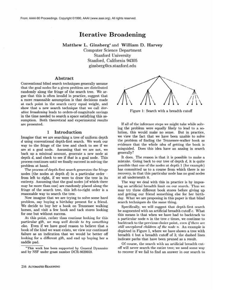
Figure 1: Search with a breadth cutoff
If all of the inference steps we might take while solving the problem were equally likely to lead to a solution, this would make no sense. But in practice,
we view the fact that we have been unable to solve
the problem of finding the Tennessee-walker book as
evidence that the whole idea of getting the book is
misguided. Does this idea have an analog in search
generally?
It does. The reason is that it is possible to make a
mistake. Going back to our tree of depth d, it is quite
possible that one of the nodes at depth 1 (for example)
has committed us to a course from which there is no
recovery, in that this particular node has no goal nodes
at all underneath it.
The way we deal with this in practice is by imposing an artificial breadth limit on our search. Thus we
may try three different book stores before giving up
and getting our friend something else for her birthday. What we are proposing in this paper is that blind
search techniques do the same thing.
Specifically, we will suggest that depth-first search
be augmented with an artificial breadth cutoff c. What
this means is that when we have had to backtrack to
a particular node n in the tree c times, we continue to
backtrack to the previous choice point, even if there are
still unexplored children of the node n. An example is
depicted in Figure 1, where we have shown a tree with
breadth 4 but a breadth cutoff of 3; the dashed lines
indicate paths that have been pruned as a result.
Of course, the search with an artificial breadth cutoff will never search the entire tree; we need some way
to recover if we fail to find an answer in our search to
depth d. We will suggest that the most practical way
to deal with this problem is to gradually increase the
breadth cutoff. So we first start by searching the tree
with an artificial breadth cutoff of 2, then try with a
breadth cutoff of 3, and so on, until an answer is found.
We will refer to this technique as “iterative broadening,” borrowing terminology from Korf’s notion of iterative deepening [Korf, 19851.
We will show in this paper that given reasonable
assumptions about the distribution of the goal nodes
along the fringe, this technique leads to tremendous
expected savings in the amount of time needed to
search the tree. The reason, roughly speaking, is that
the searches with limited breadth retain a reasonable
chance of finding a goal node while pruning large fractions of the complete space and enabling us to backtrack past early mistakes more effectively. Even if the
preliminary searches fail to find a goal node, the time
spent on them is often sufficiently small that overall
performance is not much affected.
The outline of this paper is as follows: In the next
section, we present a mathematical analysis of the technique, computing the utility of a search with breadth
cutoff c in a space of branching factor b. In Section
3, we discuss the ratio of the time needed by our approach to that needed by the conventional one for various choices of b and d, and for various densities of goal
nodes at the fringe of the tree. We present both theoret ical values (which incorporate some approximations
made in Section 2) and experimental results.
In Section 4, we show that the inclusion of heuristic information makes our met hod still more powerful,
and also that it remains viable when used in combinat ion with other search techniques (dependencydirected backtracking, etc.). Related work is discussed
in Section 5.
2
Formal analysis
Suppose that our tree, of uniform branching factor b
and depth d, has g successful goal nodes distributed
along the fringe. What we will do is assume that decisions made at each point in the search are equally
important - in other words, that there is some constant s such that if n is a node under which there is
at least one goal node, then n has exactly s successful
children. (We are calling a node successful if it has
at least one goal node somewhere under it.) The fact
that s is independent of the depth of n is the formal
analog of our claim that decisions made at different
depths are equally important. We assume that the s
successful children are randomly distributed among the
b children of n.
Since the root node is successful, it is not hard to see
that there are sd goal nodes in the tree as a whole, so
that we must have s = g ‘id. In what follows, we will
generally assume that s is an integer (so that we can
evaluate the expressions that follow), and that s > 1
(so that there is more than a single goal node on the
fringe).
Now suppose that we fix b, s and a breadth cutoff
c. For a given depth d, we will denote the probability
that the restricted-breadth search finds at least one
goal node by p(d), and the number of nodes examined
by this search by t(d). We begin by computing p(d) =
1 - p(d). What is the probability that the search fails
to find a goal node at depth d?
For d = 0 (the root node), we clearly have ;is(0) =
0. For larger d, suppose that we denote by pr(i) the
probability that of the s successful children of a node n,
exactly i of them are included in the restricted search
of breadth c. Now the probability that the search to
depth d + 1 fails is given by
f$d + 1) = x
pr(i)p(d)i
(1)
since in order for the search to fail, the depth d search
under each of the i successful children of the root node
must also fail. We sum over the various i and weight
the contributions by the probability that the i successful nodes at depth 1 all actually fail.
We can evaluate pr( i) by noting that in order for
there to be exactly i successful nodes in the restricted
search, we much choose i successful nodes from the
s that are available, and also c - i unsuccessful nodes
from the b-s available. Since the total number of
to choose the c nodes in the restricte d search from the
b present in the entire tree is given by (,“) , it is not
hard to see that
This expression, together with (l), allows us to compute p(d) for various d.
What about t(d), the number of nodes examined by
the restricted search to depth d? We begin by defining
t,(d) to be the number of nodes examined on average
by the restricted search to depth d provided that the
restricted search is successful. We immediately have
t(d) = [l - F(d)]&(d) + p(d) (cd;:;
‘>
(2)
since the complete tree of breadth c and depth d must
be searched if the restricted search fails.
We also need pr, (i), the probability that exactly i
of the depth 1 nodes are successful given that the restricted search succeeds. Bayes’ rule gives us
= El - p(d - l>ilPr(i>
1 - WI
PI+)
To complete the calculation, we need to know that
if we have c nodes at depth 1, of which i are successful,
then the average number of these c nodes we need to
examine before finding j of the successful ones is given
bY
dc + 1)
i+l
prs(i) = pr(ils) =
pr(sli)pr(i)
GINSBERGAND HARVEY 2 17
Given that the restricted search is successful, how
many of the nodes do we need to examine before finding one that is successful with the breadth cutoff c? If
i nodes are successful, and each successful node has a
probability of failure given by p, then the number of
the c nodes we can expect to examine is given by
i-l
,.
NC + 1) $0
branching
factor
4
6
9
12
15
I-\
-a
depth
4
7
11
1.9
5.9
19.8
15
59.9
1.7
1.4
1.2
5.8
4.9
4.1
20.2
17.4
14.6
55.2
46.7
38.7
1.0
3.5
12.4
32.6
Figure 2: Performance improvement for s = 2
The rationale for this expression is as follows: Each
term represents the number of nodes examined assuming that the first j successful nodes fail (which happens
with probability j? for each) and the j + 1st succeeds.
The terms are weighted by l/(1 - 8) because j? is
the probability that none of the i nodes succeeds, and
this is eliminated by our assumption that the restricted
search is successful.
Given this result, the number of failing nodes examined at depth 1 is f (i, jj) - 1 and t, (d + 1) is therefore:
1+
~Pr,(~)fGJ$d))
i
- 1
&+l
-1
I( )
C-l
+ km
(4)
The first term corresponds to the fact that the root
node is always examined; the final term t,(d) is the
number of nodes examined below the depth 1 node
that eventually succeeds. The summation is, as usual,
over the number of successful children at depth 1; for
each value of i, we compute the expected number of
failing nodes examined at depth 1 and realize that each
of these failing nodes leads to a complete search of
breadth c and depth d.
Using (1) and the expression for t, (d + 1) in (4)) we
can easily compute the probability of success and expected time taken for the first pass through the search
tree, with breadth cutoff c = 2.
Unfortunately, we cannot use these expressions to
evaluate the probabilities and time taken for subsequent searches with c = 3 and higher. The reason
is that when we do the search with c = 3, we know
that the search with c = 2 has already failed. Assuming that we do not reorder the children of the various
nodes when we iterate and search the tree again, we
need to take the fact that the c = 2 search has failed
into account when analyzing c = 3.
For f < c, let us denote by $c, f) the probability
that the search with cutoff c fails given that the search
with cutofl f is known to fail. Now it is obvious that
s4
= F(c7 f E(f)
so that we immediately have
jj(c , f) = FCC)
P(f)
(5)
We also need to do something similar for t. We will
assume (wrongly) that the expected number of nodes
218 AUTOMATEDREASONING
branching
factor
4
4
6
2.9
3.9
9
3.4
7
26.2
30.7
24.3
12
15
2.9
2.4
19.0
15.5
depth
11
451.3
292.3
186.0
129.0
97.3
15
7276.6
1990.3
928.1
559.9
390.2
Figure 3: Performance improvement for s = 3
examined during a successful search to depth d is unchanged by the fact that the search with breadth cutoff f has failed. In practice, it is possible to reorder
the nodes so that the expected number is less than
this. However, this may not be desirable because it
will abandon heuristic information present in the original order; it is because of these competing reasons that
we are taking the number to be unchanged. As in (2),
this leads to
t(c, f) = [l - F(c, f
)IW) + Pk, f)
c-l
rd+l-lJ
*
The hard work is now done. The expected time
taken to solve the problem using iterative broadening
is given by
xB(i
- l)t(i, i - 1)
(6)
where the term being summed corresponds to the time
taken by the search of breadth i, given that the previous search has failed to solve the problem.
3
Results
Theoretical
Given the results of the previous section, it is straightforward to compute the expected time taken by an
iterative-broadening search and compare it to the expected time taken by a simple depth-first search (i.e.,
c = b) . The tables in Figures 2 and 3 do this for s = 2
and s = 3 respectively and for various choices of b
(branching factor) and d (depth of tree). The numbers
appearing in the table are the ratios of these two times
and indicate the factor saved by the new approach.
(Thus the 15.5 appearing in Figure 3 for b = 15 and
d = 7 indicates that iterative broadening will typically
solve the problem 15.5 times faster than depth-first
search.)
It can be seen from these figures that iterative broadening outperforms conventional search for s 2 2 and
d >_ 4. (For shallower searches, this was not always
the case. The worst case examined was s = 2, b =
15, d = 2, when iterative broadening was 0.4 times
as fast as depth-first search.) Furthermore, as the
depth of search increases, so does the time saved. For
large depths and branching factors, it appears that
the iterative broadening technique reduces the time
needed to solve the problem by an overall factor approximately linear in b and additionally reduces the
effective branching factor by s - 1.
Note that if s were known in advance, the reduction
in effective branching factor could also be achieved by
working with a breadth cutoff of b - s + 1, since this
breadth cutoff will never prune all of the goal nodes
from the search space. Iterative broadening achieves
this savings without advance information about the
size of s. Additional savings are also obtained because
of the possible success of the searches with narrower
breadth cutoffs.
The large depth limit In the large d limit, it is
possible to use these results to determine general conditions under which iterative broadening leads to computational speedups.
As a preliminary, we can use (4) to find the expected
time needed by conventional depth-first search, obtaining for large d
bd+l(b - s)
tdf(d) = (b - 1)2(s + 1)
The time needed by iterative broadening is bounded
by the time needed for complete searches with breadth
cutoffs up to b + s - 1. We set E = s - 1 to get
Setting t(d) = tdf(d) and solving for E gives us E =
b/2d so that s = 1 + E = 1 + b/2d and the number of
goal nodes is
d
= eb/2
Proposition
3.1 In the large depth limit, iterative
broadening will lead to computational
speedup whenever the total number of goal nodes at the fringe exceeds
eb/2 .
Experimental
In order to ensure that the approximations made in
Section 2 not invalidate our theoretical results, we compared the iterative-broadening approach to conventional depth-first search on randomly generated problems. The experimental results appear in Figure 4 and
depth
3
4
5
6
7
I
1
0.5
0.4
0.5
0.4
0.5
1.5
0.7
0.8
1.1
0.9
1.3
;
0.8
1.8
2.1
2.3
4.7
2.5
1.3
2.2
3.4
3.0
6.5
3
1.5
3.3
5.1
15.2
19.5
Figure 4: Performance improvement observed
branching factor 6 and small s (100 samples)
depth
3
4
5
6
m
1
0.6
0.7
0.9
0.9
1.1
1.5
0.8
1.1
1.7
1.5
2.3
;
1.7
2.7
4.6
8.8
12.1
2.5
1.6
6.6
8.7
18.5
17.8
for
3
2.3
5.4
11.3
37.9
45.0
Figure 5: Performance improvement observed for
branching factor 6 with heuristic information (100 samples)
are in overall agreement with our theoretical expectations.
The experimental data also includes values for s
other than 2 and 3, since in practical applications a
successful node may not have-a fixed number of successful children. Data is shown for s = 1.5 and s = 2.5,
and s = 1 as well.
The case s = 1 is exceptional because it leads to exactly one goal node. Since this goal node is randomly
located on the fringe of the search tree, the fastest
search is the one that examines the fringe most rapidly,
and we can therefore expect depth-first search to outperform iterative broadening in this case. At worst, iterative broadening might be a factor of b slower (since
there are b possible iterations); in practice, we observed
only a factor of 2. This was roughly independent of the
breadth and depth of the search.
4
Heurist ii informat ion
The experiment al work described in Section 3 was
also extended to consider cases in which heuristic information is used to order the children of any particular
node so that subnodes that are likely to lead to solutions are examined first. We simulated a fairly weak
heuristic that scaled by a factor of 2(b + 1 - i)/(b + 1)
the probability that the ith child of a successful node
was itself successful. Thus the probability of the first
child’s success is approximately doubled and the probabilities for subsequent children are scaled by a linearly
decreasing amount. The results are reported in Figure
5 and indicate that heuristic informat ion improves the
relative performance of iterative broadening with respect to standard search techniques. (In fact, for b >5
GINSBERGAND HARVEY 219
and d > 6, iterative broadening is the technique of
choice even if s = 1.)
These results can be understood by realizing that
at any node, both search techniques examine the most
likely children first. The consequences of making a
mistake are different, however - if depth-first search
examines an unsuccessful node near the top of the tree,
it will go on to examine the entire subtree of that node
at potentially devastating cost. Iterative broadening
limits the fruitless search to a subtree of breadth c;
the better the heuristic, the more likely it is that a goal
will be encountered for small c. Even for the relatively
weak heuristic used in our experiments, large relative
performance improvements were obtained.
Combination with other techniques Finally, we
tested the iterative-broadening technique by including it in a program designed to create crossword puzzles by filling words into an empty frame [Ginsberg
et al., 19901. This program uses a variety of techniques, including a heuristic ranking of the children of
the node being examined, directional arc-consistency
[Dechter and Pearl, 19881, backjumping (a simple form
of dependency-directed backtracking) [Gaschnig, 19791
and dynamic search rearrangement.
The results were as expected. Performance improved
in almost all cases; the single exception was for a 5 x
5 puzzle containing 5 5-letter words in each direction
(i.e., no black squares at all). The depth of this puzzle
was shallower than for most of the others (there are
only 10 words to fill in), the branching factor is very
large (due to the large number of 5-letter words in the
dictionary) and the solutions are quite sparse in the
search space (leading to a very small value of s). As
can be seen from Figures 1 and 2, all of these factors
combine to reduce the effectiveness of the technique we
are proposing.
5
Iterative
Related
work
deepening
An attractive feature of iterative broadening is that
it can easily be combined with iterative deepening,
the most effective known technique for searching trees
where the depth of the solution nodes is unknown
[Korf, 19851. Iterative deepening works by searching
the tree to progressively larger fixed depths; any of
these fixed-depth searches can obviously be performed
using iterative broadening instead of the simple depthfirst search proposed in [Korf, 19851.
Parallel
search
Kumar and Rao have recently suggested that the most
effective way to search a tree of the sort we have been
examining is to interleave n parallel searches for the
first n children of the root node, and have shown that
this technique reduces expected search time if the dis220 AUTOMATEDREASONING
tribution of the goal nodes is nonuniform along the
fringe of the tree.
This approach works for exactly the same reason as
iterative broadening - the cost of making a mistake
is minimized. Iterative broadening can be expected to
lead to still further improvements, since parallel search
cannot address difficulties arising from mistakes made
below the first level of the search tree or from damage
done if the first n children are all failing nodes.
6
Conclusion
Iterative broadening leads to computational speedups
on search problems containing in excess of 40,000 nodes
if either s > 1.5 (so that a successful node has, on average, at least 1.5 successful children) or there is heuristic informat ion available indicating conditions under
which a node is likely to lead to a solution. In the
large depth limit, speedups can be expected whenever
there are at least ebj2 solutions to the problem in question. Since the size of the fringe grows ex onentially
with the difficulty of the problem (and ebP2 doesn’t),
we can expect this condition to be satisfied for almost
all problems that admit multiple solutions.
The speedups gained by our approach are often several orders of magnitude; this easily outweighs the cost,
which appears to be at most a factor of 2. These theoretical results are confirmed by experimentation on
both randomly generated small problems and the large
toy problem of crossword puzzle generation.
Acknowledgement
We would like to thank Bob Floyd and Rich Korf for
various helpful suggestions.
References
[Dechter and Pearl, 19881 Rina Dechter and Judea
Pearl. Network-based heuristics for constraintArtificial
Intelligence,
satisfaction problems.
34:1-38, 1988.
[Gaschnig, 19791 John Gaschnig.
surement
gorithms.
and
Analysis
of
Performance
MeaCertain
Search Al-
Technical Report CMU-CS-79-124,
Carnegie-Mellon University, 1979.
[Ginsberg et al., 19901 Matthew L. Ginsberg, Michael
Frank, Michael P. Halpin, and Mark C. Torrance.
Search lessons learned from crossword puzzles. In
Proceedings of the Eighth National
Artificial Intelligence,
1990.
Conference
on
[Korf, 19851 Richard E. Korf.
Depth-first iterative
deepening: An optimal admissible tree search.
Artificial Intelligence,
27:97-109, 1985.
