From: AAAI-97 Proceedings. Copyright © 1997, AAAI (www.aaai.org). All rights reserved.
Symbolic
Nearest
Piew Datta
Department
Mean
Classifiers
and Dennis
Kibler
of Information and Computer
University of California
Irvine, CA 92717
{pdatta, kibler}@ics.uci.edu
Figure la.
Abstract
The minimum-distance
classifier
summarizes
each
class with a prototype
and then uses a nearest neighbor approach
for classification.
Three drawbacks
of
the original minimum-distance
classifier are its inability to work with symbolic
attributes,
weigh attributes,
and learn more than a single prototype
for
each class. The proposed solutions to these problems
include defining the mean for symbolic attributes,
providing a weighting metric,
and learning several posThe learning algosible prototypes
for each class.
rithm developed to tackle these problems, SNMC, increases classification
accuracy by 10% over the original
minimum-distance
classifier and has a higher average
generalization
accuracy
than both C4.5 and PEBLS
on 20 domains from the UC1 data repository.
Science
+++
+++++
+++
+++
Figure lb.
+++
++
++++
++*+
++
++
+@ ,”
+++
63
__
pi __
0--___
+o C++
++
__
i __
0_____
++
+-I-+++
+++
++++
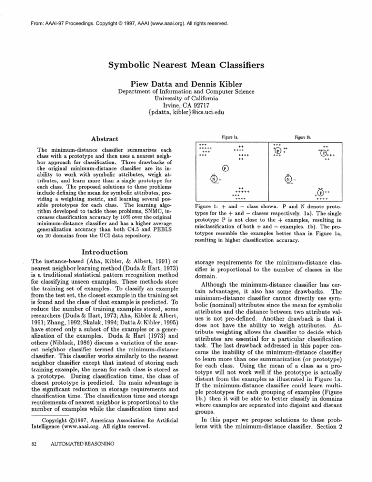
Figure
1: + and -
class
types for the + and prototype
&+
i-+-i-+
shown.
classes
P is not close
P and N denote
respectively.
to the
la).
+ examples,
proto-
The single
resulting
in
lb). The prototypes resemble the examples better than in Figure la,
resulting in higher classification accuracy.
misclassification
of both + and -
examples.
Introduction
The instance-based
(Aha, Kibler, & Albert, 1991) or
nearest neighbor learning method (Duda & Hart, 1973)
is a traditional statistical pattern recognition method
for classifying unseen examples. These methods store
the training set of examples.
To classify an example
from the test set, the closest example in the training set
is found and the class of that example is predicted. To
reduce the number of training examples stored, some
researchers (Duda & Hart, 1973; Aha, Kibler & Albert,
1991; Zhang, 1992; Skalak, 1994; Datta & Kibler, 1995)
have stored only a subset of the examples or a generalization of the examples.
Duda & Hart (1973) and
others (Niblack, 1986) discuss a variation of the nearest neighbor classifier termed the minimum-distance
classifier. This classifier works similarly to the nearest
neighbor classifier except that instead of storing each
training example, the mean for each class is stored as
During classification
time, the class of
a prototype.
closest prototype is predicted.
Its main advantage is
the significant reduction in storage requirements and
classification time. The classification time and storage
requirements of nearest neighbor is proportional to the
number of examples while the classification time and
storage requirements
sifier is proportional
domain.
Copyright
01997,
American
Association
for Artificial
Intelligence (www.aaai.org.
All rights reserved.
In this paper we propose solutions to these problems with the minimum-distance
classifier. Section 2
82
AUTOMATED
REASONING
for the minimum-distance
clasto the number of classes in the
Although the minimum-distance
classifier has cert ain advantages,
it also has some drawbacks.
The
minimum-distance
classifier cannot directly use symbolic (nominal) attributes since the mean for symbolic
attributes and the distance between two attribute values is not pre-defined.
Another drawback is that it
does not have the ability to weigh attributes.
Attribute weighting allows the classifier to decide which
attributes are essential for a particular classification
task. The last drawback addressed in this paper concerns the inability of the minimum-distance
classifier
to learn more than one summarization
(or prototype)
for each class. Using the mean of a class as a prototype will not work well if the prototype is actually
distant from the examples as illustrated in Figure la.
If the minimum-distance
classifier could learn multiple prototypes for each grouping of examples (Figure
lb.) then it will be able to better classify in domains
where examples are separated into disjoint and distant
groups.
addresses the first problem and introduces the mean for
symbolic attributes. Section 3 shows how to weigh attributes and introduces an algorithm SNM (Symbolic
Nearest Mean) that uses symbolic attributes and atSection 4 describes an extension,
tribute weighting.
SNMC, to the minimum-distance
classifier for learning
multiple prototypes for classes. SNMC uses clustering
to find groupings of the examples for each class. In
section 5 we compare these methods with C4.5 (QuinIan, 1993), PEBLS (Cost & Salzberg, 1993), and the
minimum-distance
classifier using generalization accuracy as our comparison metric. Our empirical results
show that SNMC classifies on average better than C4.5
and PEBLS. Section 6 summarizes our contributions
and describes directions for future work.
Symbolic
Attributes
The distance metric for the nearest neighbor and
minimum-distance
classifier is crucial to their predictive capabilities.
Euclidean distance, a commonly used
metric, is defined as
where z and y are two examples, a is the number of
attributes and pi refers to the ith attribute value for
example x. For real-value attributes d( xi, yi) is defined
as their absolute difference (ie. jxi - yi I).
For symbolic attributes the distance between two
values is typically defined as d(zi, yi) = 0 iff xi = yi
and 1 otherwise. This assumes that each different symbolic value is equi-distant from another.
This leads
to problems in situations where two different values
should be considered the same, and in situations where
symbolic values should have varying distances among
them. In addition, since the minimum distance classifier stores means for each class, a method for computing the mean of symbolic attributes needs to be
developed.
The most obvious method is to store the
most common symbolic value as the mean, however
this is incorrect if attribute values can have varying degrees of dissimilarity.
Although these two approaches
for determining the distance between symbolic values
and finding class means are obvious, they have their
limitations.
Distances
Values
between
Symbolic
Attribute
Stanfill & Waltz (1986) developed the Value Distance
Metric (VDM) as a method for computing different distances among symbolic values in a supervised learning
task. The VDM has two components,
weighing attributes denoted W and finding the distance between
two values denoted D. The VDM is not an actual
metric since the W component is not symmetric.
We
only use the D portion of the VDM which is similar
to MVDM (Cost & Salzberg, 1991). MVDM is based
on the ratio of the probability of the value occurring
in each class. D(v, w) is defined by
where v and w are two values from an attribute, C
is the number of classes, Ci is the ith class, S, is the
set of examples that have the value v for attribute A,
f(Ci, Sv) denotes the number of examples with class
Ci in the set S, , and 1S, 1 is the number of examples
in Sv. Note that each fraction is between 0 and 1 and
thus each difference term will be between 0 and 1. The
final distance D( x, y) can be divided by the number of
classes C so that the distance between any two values
is always between 0 and 1. Since the distance between
symbolic attribute values is bounded between 0 and 1,
dividing all real values by the range of the real-value
attribute (e.g. m~~~~a,) in the training set normalizes them2. In domains where both types of attributes
are used, the distances for them are then relative and
comparable.
All of the distances between symbolic attribute values are calculated once and stored in the
VDM table before learning takes place.
The Mean
of Symbolic
Attributes
The simplest method for determining the mean of a
symbolic attribute is to choose the most common value;
however, this does not always yield the best classification accuracy. In addition, we assume the mean of a
symbolic attribute must be one of its possible values.
For numeric data the mean is the value that minimizes
the variance. We generalize this notion to deal with
symbolic attributes as well. We define the mean of a
set of symbolic values by finding the value of p minimizing the variance, that is
where J is the set of values and v is a symbolic value
in J. p will act as the best constant approximation
for the symbolic values in J similar to the mean for
real values. Computationally,
each symbolic value will
be tried as p and the symbolic value that minimizes
the variance will become the mean for J. We define
the mean of a set of examples, S, to be the vector
< Al,, A2,, . . .An, > where Ai, denotes the mean of
the ith attribute. We call this vector the prototype for
s.
We have developed an algorithm called SNM (Symbolic Nearest Mean) that has a more robust method for
determining distances between symbolic values. SNM
uses the MVDM and the definition of mean described
above. If missing values occur in the training set, they
are replaced by the most common value of the attribute
in the class. SNM learns a prototype for each class,
classifies examples by finding the closest prototype using Euclidean distance, and predicts the prototype’s
class. If a missing value occurs in a test example, the
21f the range of the attribute
in the test set is larger
than the maximum value in the training set the test value
is set to 1.
CLASSIFICATION
83
attribute
example.
is not used to compute
Attribute
the distance
for the
Weighting
Inferring the applicability
of an attribute is important for classification.
The minimum-distance
classifier
weighs all of the attributes equally which may decrease
One way of introducing
atclassification
accuracy.
tribute weighting to the minimum-distance
classifier is
through the MVDM. Since the distances between symbolic values can vary, the MVDM provides a method
for weighing symbolic attributes based on classification
relevance.
For example, if the distances between the
values for symbolic attribute A only range from .Ol to
.02 then this attribute has less weight than symbolic
attribute B which has distances varying from 0.7 to
0.9. Thus the MVDM is indirectly showing A to be
less relevant than B for classification.
One advantage of using the MVDM is that it weighs
symbolic attributes based on the distributions of their
values in the different classes. The MVDM provides
a more precise weighing method than simply stating
that an attribute has a particular weight; it weighs
each value of the symbolic attributes.
Thus far SNM
does not weigh real-value attributes. A simple method
of weighing real-value attributes is to discretize them
and use the MVDM to define the distances between
each of their new discretized values.
It may seem unintuitive to discretize real-value attributes since nearest neighbor type algorithms are
However,
naturally suited to real-value attributes.
these distances do not necessarily reflect the usefulness of the values for classification.
For example, suppose we have a real-value attribute denoting the average number of cigarettes a person smokes daily. Intuitively there is a large difference between person A
who smokes 0 cigarettes and person B who smokes 1
cigarette even though the actual difference between the
number of cigarettes for these two people is 1. The
difference between the number of cigarettes person C
smokes (say 10) and person D (say 11) is also 1. Although the actual difference between each pair of these
cigarette smokers (A & B versus C & D) is 1 , for classification purposes we would want a large difference
between persons A and B and a small difference between persons C and D.
Experiments
Applying
Discretization
To test our hypothesis that discretizing real-value attributes would increase the classification accuracy of
SNM, we compared its classification performance with
discretization and without. We applied a discretization
process that orders the attribute values and creates intervals for the corresponding symbolic values such that
the intervals contain an approximately
equal number
of examples.
Results in Dougherty, Kohavi, & Sahami(1995)
suggest that 10 intervals are satisfactory
84
AUTOMATED
REASONING
Table 1: Accuracy comparison on SNM with discretization vs. without discretization.
(* indicates a statistical significance at the 95% level or higher using a
two-tailed t-test)
SNlU
DOKXlZliIl
w/o
Breast Can.
Breast Can. Wis.
Credit
Flag
Glass
Heart Disease
Hepatitis
Iris
Pima Ind. Dia.
Waveform
Wine
Discr.
66.0%
95.7%*
84.8%
55.7%
43.9%
83.6%
78.6%
91.5%
72.8%
80.5%
95.2%
w/
Discr.
69.9%”
91.6%
85.0%
69.5%”
60.2%*
83.2%
81.9%*
91.4%
72.9%
81.6%”
95.8%
and after some initial experiments, we felt that 10 intervals also works with our discretization process. Intuitively, if we create too many intervals (more than
necessary for maximum accuracy),
then the MVDM
will tend to give zero distance to intervals that should
be merged. If too few intervals are created, however,
the MVDM has no way of separating the intervals.
Therefore, the MVDM is more forgiving if slightly too
many intervals are created rather than too few.
Table 1 shows the results of 30 runs of this experiment randomly choosing two-thirds of the examples
(without replacement) as training examples and the remainder as test examples3 on 11 domains from the UC1
Data Repository (Murphy & Aha 1994) containing either a mixture of symbolic and real-value attributes
or only real-value attributes.
Both the training and
test sets retain the original class probabilities.
The
table shows that in almost all domains, (except the
Breast Cancer Wisconsin domain which appears to be
discretized in its original form), discretization
aids in
classification accuracy (an * indicates a statistical significance at the 95% level or higher using a two-tailed
t-test) or does not decrease accuracy significantly.
In
some domains the increase is not great; however, in
others it considerably boosts the accuracy of SNM. By
weighing the real-value attributes through the MVDM,
SNM now has a method of choosing the more relevant
attributes for classification.
Therefore, we will adopt
the discretization of real-value attributes in SNM.
3We realize that the testing sets in the 30 runs are not
independent;
however, we apply the t-test as a heuristic to
show that the two accuracies can be considered
different.
Kohavi( 1995) recommends
multiple runs of cross validation, but we contend that this methodology
suffers from
the same independence
problem.
Learning
Multiple
Prototypes
The last drawback of the minimum-distance
classifier
is that it works best on domains where there is one
prototype for each class. The classification
accuracy of
SNM and the minimum-distance
classifier decreases as
more classes require multiple prototypes to represent
the examples. Using more than one prototype per class
allows this method to represent distant and disjoint
groups of examples within the classes. The difficulty
lies in determining
the grouping of examples for the
prototypes.
One possible approach to finding groups of examples in the same class is clustering.
Typically clustering is used in an unsupervised
environment
for data
Since the examples in an unsupervised
exploration.
environment
are not presorted into groups, there is no
clear metric to optimize. In our classification
task the
examples are presorted by class, but we want to find
clusters within each of the classes. One way to judge
whether a reasonable number of clusters are found in a
class is to check the classification
accuracy of all trainClassification
accuracy can be used as
ing examples.
a heuristic for determining
the number of clusters in
individual classes.
The next section describes the method adopted by
SNMC (Symbolic
Nearest Mean with Clustering),
our
modification
to SNM for representing
multiple prototypes within classes. First we describe k-means clustering and then describe a method of deciding on Ic,
the number of clusters for each class.
K-Means
Clustering
An area in statistics
and machine learning called
clustering focuses on the unsupervised task of finding
groupings of examples. An efficient algorithm for partitioning a set into L clusters is k-means clustering (Duda
& Hart, 1973; Niblack, 1986; MacQueen,
1967). Figure 2 shows the algorithm for k-means clustering. The
two main parameters to this algorithm are the distance
metric for finding the closest cluster and k, the number
of clusters to create.
Euclidean distance is the most
commonly
applied distance measure, although other
distance metrics do exist such as city block distance
and Mahalanobis
distance (Duda & Hart 1973).
Finding Ic, on the other hand, is a more serious
Duda & Bart, Smyth(1996),
Cheeseopen problem.
Randomly initialize k: clusters.
Repeat
Compute cluster means.
For each example
if closest cluster to ex. # current
move ex. to closest cluster
Until (no exs. have moved)
Figure
2: Pseudocode
For each class c
I%,= 1.
Repeat
For each class c
If (Ic, + 1 improves accuracy)
then learn one additional
Until (accuracy has not improved)
Learn prototypes for each cluster.
Figure
for k-means.
of ex.
for c.
for SNMC.
man & Stutz(1988),
Schmidt et. al. (1994) and other
researchers have suggested various methods to determine the number of clusters in a group of examples;
however these are all for learning in an unsupervised
environment.
Finding
Training
the Number
Set Accuracy
of
Clusters
through
Although learning several clusters for each class seems
similar to the clustering paradigm, we do have class
information
available.
Although class information
is
not helpful in creating the clusters (since all examples
will be from the same class), it can help to restrict the
number of clusters to create. SNMC uses the accuracy
on the training set as a feedback mechanism for learning a vector I%where Ici is the number of clusters for
class i. The general idea behind SNMC is to create
more clusters in a particular
class if it increases the
classification
accuracy of the prototypes
representing
the training examples. The bias in SNMC is to create
as few clusters as possible, but to increase I%i when it
leads to an increase in accuracy.
Figure 3 shows the procedure for SNMC. SNMC uses
a hill-climbing
search method.
It temporarily
increments the number of clusters in each class to see if
the classification
accuracy on the training set has increased.
Ici is only incremented
if it results in an increase in classification
accuracy on the training set.
SNMC separates the training examples by class and
then attempts to find clusters that maximize classification accuracy on the training examples4.
Afterwards
SNMC learns prototypes for each cluster in the same
manner as SNM. SNMC predicts classes for unseen test
examples by finding the closest prototype and predicting the class of the prototype.
Evaluation
cluster
3: Pseudocode
cluster
of the SNM
and SNMC
To evaluate the applicability of these concept
tions to the classification
task, we compared
descripthe ac-
4SNMC calls k-means 5 times with the same I;i and
chooses the set of clusters returned from k-means with the
highest classification
accuracy to represent the accuracy of
L,. This helps to overcome the dependency
k-means has on
an initial random state.
CLASSIFICATION
85
curacy of SNM and SNMC with C4.5, PEBLS and
the minimum-distance
classifier. We compared these
algorithms on 20 domains from the UC1 Repository.
Three of these domains are artificial (LED domains
and Hayes Roth) and the remaining are real world domains. These domains have a variety of different characteristics including different types of attributes, and
a large range in the number of examples, attributes,
and classes.
We describe the methodology
for this evaluation.
We ran 30 tests randomly picking without replacement
two-thirds of the data as the training set and using the
remainder as the test set5 in each of the domains 6
and compared the average accuracy of C4.5, PEBLS,
the minimum-distance
classifier (Min-dis.),
SNM, and
SNMC. These results are shown in Table 2. The table
represents the accuracy f the standard deviation followed by the rank of the algorithm; the algorithm with
the highest accuracy has rank 1. The average accuracy
and average rank of each of the algorithms are shown
at the bottom of the table. The average accuracy gives
relative ratings of the algorithms taking into consideration the magnitude of difference in accuracy while the
average rank disregards the magnitude.
SNMC has the highest average accuracy in all of
these domains with PEBLS and C4.5 coming in second and third respectively.
SNMC has an average increase in accuracy of at least 2% over C4.5 and PEBLS.
SNMC also has the best rank of all of the algorithms
(2.1); PEBLS and SNM are tied for the next best rank.
SNM has a average accuracy slightly lower than C4.5
although not much lower. In fact, considering the simplicity and efficiency of SNM, it classifies surprisingly
well. Similar results have been seen with other simple
methods (Auer, Holte, & Maass, 1995; Iba & Langley,
1992). The minimum-distance
classifier has the lowest
average accuracy and rank of all the algorithms. The
proposed solutions for the three problems described in
this paper result in almost a 10% increase in accuracy
from the minimum-distance
classifier to SNMC.
When comparing
SNMC with C4.5 and PEBLS,
SNMC has a higher accuracy than C4.5 in 13 of the 20
domains and has a higher accuracy than PEBLS in 12
of the 20 domains.
Applying a single Wilcoxon test,
the null hypothesis that C4.5 and SNMC have equal
average accuracies over all of the domains is rejected
at the 95% significance level. When applying a single
Wilcoxon test to PEBLS and SNMC, the null hypothesis is rejected at the 95% significance level. According
to the Wilcoxon
test, SNMC is significantly different
than C4.5 and PEBLS and the average accuracy of
SNMC shows it is more accurate than C4.5 and PEBLS
over these 20 domains. For details on additional experimental evaluation refer to Datta & Kibler (1997).
Contributions
and
ture Work
The first important contribution of this paper is identifying three problems
with the minimum-distance
classifier, namely its inability to work with symbolic
attributes,
weigh attributes,
and learn disjunctions
within classes. This paper describes two algorithms,
SNM and SNMC. These algorithms share some core
features such as the method they use to define the
mean of a cluster, their distance metric, and discretization of real-value attributes.
SNMC extends SNM by
being able to learn multiple prototypes for classes by
applying k-means clustering. The experimental results
show that they perform comparable to both C4.5 and
PEBLS in the classification task. In fact SNMC has
the highest average accuracy and the best rank in the
domains used in our experimentation.
There are several directions for future extensions to
this work. Certainly more sophisticated
methods for
discretizing real-valued attributes (e.g. Wilson & Martinez, 1997) can be applied as well as more complex
distance metrics (e.g. the Mahalanobis
distance metric). The heuristic used in SNMC could be replaced
by a cross-validation
method to find the Ici for each
class. The methods described in this paper do not use
any prior class distribution information
or weigh the
prototypes which could boost classification accuracy.
Acknowledgments
We thank Randall Read for commenting
drafts of this paper. We are also grateful
tors to the UC1 data repository.
on previous
to contribu-
References
Aha, D., Kibler, D. & Albert M. (1991).
Instancebased learning algorithms.
Machine learning, volume
6, pp 37-66. Boston, MA: Kluwer Publishers.
Auer, P., Holte, R. & Maass, W. (1995). Theory and
applications of agnostic PAC-learning with small decision trees. In Proceedings of the Twelfth International
Conference on Machine Learning.
Tahoe City, CA.
Morgan Kaufmann.
Datta, P. and Kibler, D. (1997).
Learning Multiple
In Proceedings
of the FourSymbolic Prototypes.
teenth International Conference on Machine Learning.
Nashville, TN. Morgan Kaufmann.
Datta, P. and Kibler, D. (1995). Learning Prototypical
In Proceedings of the Twelfth
Concept Descriptions.
International Conference on Machine Learning. Tahoe
City, CA. Morgan Kaufmann.
Cheeseman,
P. & Stutz, P. (1988).
AutoClass:
A
Bayesian Classification System. In Proceedings of the
Fifth International Conference on Machine Learning.
Morgan Kaufmann.
cost, s. and Salzberg, S. (1993). A weighted nearest
neighbor algorithm for learning with symbolic features.
Machine Learning, volume 10, pp. 57-78. Boston, MA:
86
AUTOMATED REASONING
Table 2: Accuracy
Domain
Audiology
Breast Cancer
Br. Can. Wis.
Cl. Heart Dis.
Credit
Flag
Glass
Hayes Roth
Hepatitis
House Votes
Iris
LED (200 exs.)
LED w/irr. feat.
Lymphography
Pima Ind. Dia.
Promoters
Soybean-large
Waveform
Wine
zoo
c4.5
88.2f4 (2)
73.ozt3
95.1&l
71.9f6
84.4f2
72.5f5
68.4f6
81.2f4
80.3f5
96.1&l
95.4f3
57.2f5
67.3f4
79.5&5
72.lrf3
78.3f7
86.8f4
74.9f.9
92.7f4
98.4f2
Ave. Accuracy
Ave. Rank
80.7
3
(1)
(2)
(5)
(3)
(1)
(2)
(3)
(3)
(1)
(1)
(4)
(3)
(4)
(4)
(4)
(3)
(5)
(5)
(4)
and Number of Prototypes
PEBLS
89.4&3 (1)
67.3f4 (4)
92.6f2 (4)
77.1*3 (4)
82.2f2 (5)
65.3f5 (4)
70.3f5 (1)
85.5f4 (1)
79.3f6 (4)
94.2&l (3)
93.7f4 (2.5)
48.3f5
(5)
62.8&4 (4)
82.9f4 (1)
69.4f3 (5)
89.0f4 (3)
92.4f2 (1)
77.7f.9
(4)
97.4-+2 (1)
100&O (1)
80.8
2.9
Kluwer Publishers.
Dougherty, J ., Kohavi, R., Sahami, M. (1995). Supervised and Unsupervised
Discretization
of Continuous
Features. In Proceedings of the Twelfth International
Conference on Machine Learning.
Tahoe City, CA.
Morgan Kaufmann.
Duda, R., and Hart P. (1973).
Pattern classification
and scene analysis. New York: John Wiley & Sons.
per Class for SNMC
Min-dis.
72.8f6
62.0f8
95.8&l
80.5f4
83.1f2
55.0f6
41.0f7
75.4f5
77.0f6
87.3&3
92.1f4
62.7f13
29.7f4
71.0f7
73.1f2
71.3f9
68.4f5
79.2&6
95.6f2
98.3f3
73.6
4.25
Quinlan,
Learning.
(5)
(5)
(1)
(3)
(4)
(5)
(5)
(4)
(5)
(5)
(5)
(3)
(5)
(5)
(3)
(5)
(5)
(3)
(4)
(5)
SNM
82.4f5
70.2f5
91.8&l
83.5f3
85.2f2
67.4&5
61.lf7
38.4f7
82.9f5
90.4f2
92.7f4
67.6f5
73.ozt3
82.1f4
75.3f3
91.4f5
82.2f4
81.lh.8
96.1f3
99.5f2
SNMC
(.3)
(3)
(5)
(1)
(2)
(2)
(4)
(5)
(1)
(4)
(4)
(1)
(1)
(3)
(2)
(1)
(4)
(2)
(3)
(3)
81.9f4
72.3f3
94.2f2
83.3f3
85.3f2
65.7f5
67.7f6
83.2f6
82.5f5
94.9*2
93.7f4
65.1f5
72.5f3
82.5f5
75.8f3
90.6rt5
86.9f4
81.4&l
97.1f2
99.7f2
79.7
2.7
(4)
(2)
(3)
(2)
(1)
(3)
(3)
(2)
(2)
(2)
(2.5)
(2)
(2)
(2)
(1)
(2)
(2)
(1)
(2)
(2)
82.8
2.1
J. R. (1993).
C4.5: Programs for Machine
Morgan Kaufmann, San Mateo, CA.
Schmidt, W. Levelt, D. & Duin, R. (1994).
An experimental comparison of neural classifiers with ‘traditional’ classifiers. Pattern Recognition in Practice IV:
Multiple Paradigms, Comparative Studies, and Hybrid
Systems, Proceedings of an International
Workshop.
Vlieland, The Net herlands, Elsevier .
Iba, W. & Langley, P. (1992). Induction of one-level
In Proceedings
of the Ninth Interdecision trees.
national Workshop on Machine Learning.
Aberdeen,
Scotland. Morgan Kaufmann.
Skalak, D. (1994).
Prototype
and feature selection
by sampling and random mutation hill climbing algorithms. In Proceedings of the Eleventh International
Conference on Machine Learning, New Brunswick, NJ.
Morgan Kaufmann.
Kohavi, R. (1995).
A study of cross-validation
and
bootstrap for accuracy estimation and model selection.
In Proceedings of the 14th International Joint Conference on Artificial Intelligence. Morgan Kaufmann.
Smyth, P. (1996). Cl us t ering using Monte Carlo CrossValidation. In Proceedings of the Second International
Conference on Knowledge Discovery and Data Mining.
Seattle, Washington.
MacQueen, J. (1967). S ome methods for classification
and analysis of multivariate observations.
In Proceedings of the fifth Berkeley symposium on mathematical
statistics and probability.
Vol. 1. University of California Press, Berkeley.
Stanfill, C., & Waltz, D. (1986).
based reasonin
Communications
29. no 12. pp. f213-1228.
Murphy, P. and Aha, D. (1994). UC1 repository of machine learning databases [machine readable data repository]. Tech. Rep., University of California, Irvine.
Niblack, W. (1986). An Introduction
Processing.
Prentice Hall.
to DigituE Image
Toward memoryof the ACM. vol.
Wilson, D. & Martinez, T. (1997). Improved Heterogeneous Distance Functions.
Journal of Artificial Intelligence Research. Vol. 6. pp. l-34.
Zhang,
J. (1992).
Selecting typical
instances
in
instance-based
learning. In Proceedings of the Ninth
International
Conference on Machine Learning, New
Brunswick, NJ. Morgan Kaufmann.
CLASSIFICATION
87
