From: AAAI-94 Proceedings. Copyright © 1994, AAAI (www.aaai.org). All rights reserved.
Epsilon-Transformat ion: Exploiting Phase Transitions to Solve
Combinatorial Optimization Problems - Initial Results*
Weixiong
Zhang
and Joseph C.
Computer Science Department
University of California, Los Angeles
Los Angeles, CA 90024
Email: {zhang, pemberto}@cs.ucla.edu
Abstract
It has been shown that there exists a transition in the
average-case
complexity
of searching
a random tree,
from exponential
to polynomial
in the search depth.
We develop
a state-space
transformation
method,
called e-transformation,
that makes use of this complexity transition
to find a suboptimal
solution.
The
expected
number of random tree nodes expanded by
branch-and-bound
(BnB)
using e-transformation
is
cubic in the search depth, and the relative error of the
solution cost compared
to the optimal solution cost is
bounded by a small constant.
We also present an iterative version of e-transformation
that can be used to
find both optimal
and suboptimal
solutions.
Depthfirst BnB (DFBnB)
using iterative e-transformation
significantly
improves upon truncated DFBnB on random trees with large branching
factors and deep goal
nodes, finding better solutions sooner on average. On
the asymmetric
traveling salesman problem,
DFBnB
using e-transformation
outperforms
a well-known
local search method,
and DFBnB
using iterative
etransformation
is superior to truncated
DFBnB.
Introduction
It has been observed that phase transitions
exist in
many intelligent
systems (Huberman
& Hogg 1987)
and combinatorial
problems (Cheeseman,
Kanefsky, &
Taylor 1991; Karp & Pearl 1983; McDiarmid 1990; McDiarmid & Provan 1991; Mitchell, Selman, & Levesque
1992; Zhang & Korf 1992; 1993; 1994). A phase transition is a dramatic change to some problem property as
some order parameter changes across a critical point.
For example, water changes from a liquid to a solid
when the temperature
drops below the freezing point.
The earliest evidence of computational
phase transitions was the phase transition of a tree-search problem
(Karp & Pearl 1983), which has recently been studied
in detail (McDiarmid
1990; McDiarmid & Provan 1991;
Zhang & Korf 1992; 1993; 1994). The problem is to find
an optimal goal node of the following random tree.
*This research was supported
by NSF Grant No. IRI9119825, a grant from Rockwell International,
a GTE graduate fellowship
(1992-93),
and a UCLA Chancellor’s
Dissertation Year Fellowship
(1993-94).
Definition 1 (McDiarmid
& Provan 1991) A random
tree T(b,d) is a tree with depth d, and independent
and
identically distributed (i.i.d) random branching factors
edge costs are bounded i.i.d.
with mean b. Nonnegative
random variables. The cost of a node is the sum of the
edge costs on the path from the root to that node. An
optimal goal node is a minimum-cost
node at depth d.
Best-first search (BFS) and depth-first branch-andbound (DFBnB)
can be used to search these random
trees. Both are special cases of the general branch-andbound (BnB) technique.
See (Pearl 1984; Korf 1989;
Kumar 1992) for the details of these algorithms.
It turns out that the cost of an optimal goal node
of T(b, d), and the expected complexity
of BFS and
DFBnB
on T(b, d) experience phase transitions.
The
order parameter
that determines
these transitions
is
the expected number of children of a node whose cost
is the same as that of their parent, which are called
same-cost children. This is the same as the expected
number of zero-cost edges emanating
from a node. If
~0 is the probability
that an edge has cost zero, then
bpo is the expected number of same-cost children of a
node. When bpo increases from less than one to greater
than one, the expected cost of the optimal goal node
of T(b, d) changes from a linear function of d to a constant, and the expected time complexity of BFS and
DFBnB decreases from exponential in d to at most cubic in d. These phase transitions
are summarized
by
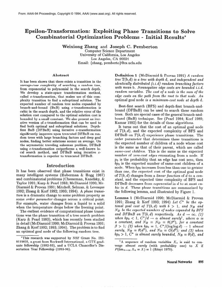
the following lemma, and illustrated by Figure 1.
Lemma 1 (McDiarmid
1990; McDiarmid
& Provan
1991; Zhang & Korf 1993; 1994) Let C* be the optimal goal cost of T(b, d) with b > 1, and NB and
ND be the expected numbers of nodes expanded by BFS
and DFBnB
on T(b, d) respectively.
As d -+ 00, (1)
where CY is
when bpo < 1, C*/d + cu almost surely’,
a constant, and NB = ND = Q(pd), for a constant
/? > 1; (2) when bp, = 1, C*/(log logd) -+ 1 almost
surely, NB = 0(d2), and ND = O(d3); and (3) when
bpo > 1, C* is almost surely bounded, NB = B(d), and
‘A
verge
sequence
of random
variables
X,
almost
suP-ely (with
probability
P&m,,,
X, = X) = 1 (RCnyi 1970).
is said to conone)
to X
if
Neural Networks
895
I
I
bw
I
1.0
I
I
I
1
optimal goal cost is
boundedby a constant
complexity is
polynomial in d
0.8 -
polynomial region
transition boundary
branching
factor b
15
optimal goal cost is linear in d
complexity is exponential in d
Figure
1: Phase
ND = O(d2).
transitions
•I
Epsilon-Transformation
&-transformation
is based on the following very simple
observation
of Figure 1. For a random tree T(b, d),
if we can increase the expected number of same-cost
children of a node so that bpo 2 1, then the expected
complexity
of finding an optimal goal node becomes
polynomial in d. This can be accomplished
by raising
the probability po of zero-cost edges, since the branching factor b is usually fixed by the structure
of the
state space. However, increasing po means obtaining a
better node-cost function (Zhang & Korf 1994), which
requires more information
about the problem, and is
By sacrificing solution quality,
generally impractical.
however, we are able to transform the problem of finding an optimal solution with exponential
average computation,
to the problem of finding a suboptimal
solution with polynomial average computation
by artificially increasing PO. This is illustrated by Figure 2.
We increase po by setting some non-zero edge costs
to zero. To reduce the amount of information lost, and
to improve the expected solution quality, we only set to
zero those edge costs that are below a particular value
Neural Networks
a difficult problem
to an easy one.
of tree search problems.
Many practical
search problems,
such as planning
and scheduling,
require computation
exponential
in
the search depth, even in the average case. However,
we usually do not need optimal solutions, but rather
ones that have a satisfactory
quality and can be found
quickly.
In this paper, we develop a state-space
transformation method, called &-transformation,
that can be used
by a search algorithm, such as BnB, to find suboptimal
solutions quickly. This method makes use of the phase
transition
in Figure 1. We analyze its average-case
We also present an iterative version of
performance.
&-transformation
for finding both suboptimal
and optimal solutions.
Finally, we evaluate the performance
of both methods on random trees and the asymmetric
traveling salesman problem.
896
Figure 2: Transform
20
E. This is why we call our method E-transformation.
E
is set to the smallest value such that a suboptimal goal
node can be found in polynomial average time.
Definition 2 For a constant E, an E-tree T,(b, d) of a
random tree T(b, d) is the same as T(b, d), except that
those edge costs in T(b, d) that are less than or equal
to E are set to zero in TE(b,d),
and the node costs are
updated accordingly.
The edge and node costs of T(b, d)
are referred to as actual values, and the edge and node
costs of T,(b, d) are called face values.
&-transformation
converts one random tree to another one with an adjusted edge-cost distribution,
i.e.,
with an increased probability
of a zero-cost edge. Let
f(x)
be the density function
and F(z)
be the distribution
of edge costs.
Then the probability
that
an edge has cost less than or equal to E is F(E) =
Jl f(t)dt, which is also the probability pE that an edge
how
of T, (b, d) has cost zero. Figure 3(a) illustrates
&-transformation
adjusts an edge-cost
density funcand its corresponding
tion. Figure 3(b) s h ows a T(2,2)
T,(2,2)
with E = 0.25, where the numbers in the nodes
and on the edges are node costs and edge costs, respectively. The optimal goal node of an g-tree is not necessarily the optimal goal node of its original tree, thus
&-transformation
is not guaranteed to find an optimal
goal node.
After the transformation,
BFS or DFBnB
can be
used to find an optimal goal node of TE (b, d), and return
the actual value of this goal node. For simplicity, we
call BnB, BFS, or DFBnB
using E-transformation
EBnB, E-BFS, or E-DFBnB,
respectively.
In order for E-BnB to run in polynomial
average
time, the value of E is chosen such that bp, s 1. To
maximize the solution quality, we select the mmimum
E that satisfies bpE > 1. That is, we choose
&* = min{@p,
2 l},
where
pE = F(E).
(1)
When E = E*, we use the term E*-transformation.
The
performance
of E*-transformation
is summarized
by
the following theorem.
initial edge-cost density
original random tree
n
adjusted edge-cost density
optimh goal node
(a) adjust an edge-cost density
Figure
3: An example
(b) transform a random tree
of e-transformation.
Theorem
1 On a random tree T(b, d) with bpo < 1,
as d -+ 00, E*-BnB runs in expected time that is at
most cubic in d, and finds a goal node whose relative
solution cost error ((C - C*)/C*,
where C is the solution cost and C* is the optimal solution cost) is almost surely a constant less than or equal to (S/a - l),
where a is a constant as defined in Lemma 1, and
S = E[edge cost x 1 x 5 E*].
Proof See (Zhang & Pemberton
1994). •I
A useful feature of E-transformation
is that a tradeoff can be made between
the average search efficiency and the average solution quality. Solutions with
higher (lower) average costs can be produced with
less (greater)
average computation
by using a larger
(smaller) value of E.
Learning
E and Actual-Value
Pruning
The value of E is a function of the branching factor b
and the edge-cost distribution
F. For practical probNeverthelems, b and F are generally not available.
less, the value of & can be learned on-line during search.
Consider DFBnB
as an example. If DFBnB
examines
the children of the current node in increasing order of
their face vales (node ordering), and breaks ties in favor
of a node with a lower actual node cost, then the first
leaf node reached is the same whether &-transformation
is used or not. DFBnB
can sample the branching factors and edge costs of all nodes along the path to the
first leaf node, and use them to estimate b and F. As
the search proceeds, the estimates of b and F can be
refined and used to update the value of E.
&-BnB can also use actual-value pruning, which prevents BnB from exploring an interior node if its actual
value exceeds the actual value uaV of the best goal node
found up to that point. This pruned interior node cannot lead to a goal node with an actual value less than
uaV. Intuitively,
one might expect actual-value
prun-
ing to improve the efficiency of BnB, and not to affect the solution quality. However, actual-value
pruning reduces the opportunity
to update the face-value
upper bound, consequently
causing some nodes with
higher face value to be expanded, which are not visited by &-BnB without actual-value pruning.
Overall,
&-BnB with and without actual-value
pruning explore
different parts of the search tree. Their relative effect
on runtime and solution quality depends on their relative pruning power and the specific problem instance.
Our results on random trees show that E*-DFBnB
with
actual-value pruning runs longer but finds better solutions than &*-DFBnB
without actual-value pruning.
Iterative
dhansformation
If we need a better solution than can be guaranteed
by E-transformation,
then we can use an E that is less
than E*. In order to determine the largest value of E
that satisfies a given error bound, we need to know the
optimal solution cost, which in general is not available.
We suggest an algorithmic
approach to address this
issue, which is called iterative E-BnB. Iterative &-BnB
performs a sequence of BnB searches with a series of
E-transformations,
where the value of E is reduced over
successive iterations.
The first iteration performs E*BnB. Within each iteration,
BnB keeps track of the
largest actual edge cost encountered that is strictly less
than E‘, among all those that are set to zero. Call this
if the cost
value fvmaa:. At the end of an iteration,
of the solution found is less than the required solution cost by comparing it to some lower bound, then
the algorithm stops.
Otherwise,
a new value of E is
calculated.
The algorithm is then repeated until a satisfactory solution is found.
The most conservative
way to update E is to set
5 = fvrna,. It can be easily shown that if edge costs
are integers bounded by a constant,
then iterative EBnB that uses E = fv,,,
in the next iteration expands
asymptotically
the same number of nodes as &-BnB
that uses the exact value of E for finding a solution of
required quality.
In general, however, a small reduction in the value of E may only cause a few new nodes
to be explored in the subsequent
iteration,
which in
turn may lead to a large number of iterations,
and
consequently
a large node-regeneration
overhead.
Alternatively, we may decrease the value of E by a larger
amount, such as E = fvmac/2.
Experimental
Study
In this section, we identify the conditions under which
&-transformation
and iterative &-transformation
are effective. To this end, we compare &-DFBnB
and iterative E-DFBnB
with other approximation
algorithms.
Iterative E-DFBnB
can be used in the same way as
truncated
DFBnB
(Ibaraki
et al. 1983; Zhang 1993)
to find approximate
and optimal solutions.
Truncated
DFBnB is a DFBnB that terminates prematurely when
the total available computation
has been exhausted.
Neural Networks
897
as the average solution cost for a given
performance
number of node expansions, since expanding a node is
the primary operation.
In our experiments,
the value
of E was updated to fvmac/2 after each iteration.
Figure 4 shows our results on uniform random trees
T(b = 2,d = 10) and T(b = 10, d = 20). The edge
costs are uniformly chosen from (0, 1,2,. . +, 216 - 1).
The results are averaged over 1000 trials.
The horizontal axes, on a logarithmic
scale, are the average
number of node expansions,
and the vertical axes are
the average relative goal cost error. Figure 4 indicates
that iterative &-DFBnB
without actual-value
pruning
is slightly better than with actual-value pruning. Compared to truncated DFBnB,
iterative E-DFBnB
finds a
better solution with the same average number of node
For instance, at 1000 node expansions in
expansions.
Figure 4(b), the relative error for iterative E-DFBnB
is
10.4010, while the relative error for truncated
DFBnB
is 40.4%. The results also show that when the branching factor and tree depth are increased (from Figure
further outperforms
4(a) to 4(b)), i t era t ive &-DFBnB
truncated DFBnB.
The relative advantage of iterative E-transformation
also depends on the edge-cost
distribution.
Specifically, the relative improvement in average solution cost
of &-DFBnB
over truncated
DFBnB
decreases when
the probability of a zero-cost edge is increased.
ncated DFBnB
&-DFBnB with
actual value pruning
lo2
node expansions
(a) b=2,
90
d= 10
edge costs from
(0,1,2, ....2’6-1)
-$ 80
‘5 io
9
60
truncated
DFBnB
E-DFBnB with
102
103
104
node expansions
105
Asymmetric
(b) b= 10, d=20
Figure
4: Iterative
E-DFBnB
vs. truncated
DFBnB.
The best solution found up to that point can then be
taken as an approximation.
The main difference between these two algorithms
is that the territory
explored by iterative E-DFBnB
is generally smaller than
the territory explored by truncated DFBnB,
although
iterative e-DFBnB
may re-expand a node many times.
Local search (Johnson
1990; Kanellakis & Papadimitriou 1980; Lin & Kernighan
1973) is a well-known
approximation
method for many difficult combinatorial problems.
Starting
at an initial solution, such as
one generated by a polynomial-time
approximation
algorithm,
local search continuously
improves the current solution by local perturbations,
until no further
improvement
can be made. This process may be invoked many times with different initial solutions.
A
serious drawback of local search is that it cannot determine if the best solution found so far is optimal,
unless the optimal solution cost is already known.
Random
Trees
We ran both iterative E-DFBnB
and truncated DFBnB
on the same set of random trees, and recorded the total
number of node expansions when either algorithm updated its current best solution. We then measure their
898
Neural Networks
Traveling
Salesman
ProbIem
The asymmetric
traveling salesman problem (ATSP)
is an NP-hard combinatorial
problem (Garey & Johnson 1979). Given n cities and an asymmetric
matrix
(c;,j) that defines a cost between each pair of cities, the
ATSP is to find a minimum-cost
tour that visits each
city exactly once and returns to the starting city. The
ATSP can be optimally solved by BnB, using the solution cost of the related assignment problem (AP) (Papadimitriou & Steiglitz 1982) as a monotonic heuristic
function. The state space of the ATSP under BnB is a
tree without duplicate nodes. See (Balas & Toth 1985)
for a description of the method.
In our implementation
of E-DFBnB
and iterative
EDFBnB,
we used the sampling
method
described
above to learn the value of E* for the first iteration.
In each subsequent
iteration,
the value of E was set
&-DFBnB
without
to fvmaz/2. F rom our experiments,
actual-value
pruning performs worse than &-DFBnB
with actual-value pruning, and thus we present the results of &-DFBnB with actual-value pruning.
We used many different cost matrices in our experiments. Our data shows that iterative E-DFBnB
finds
better solutions sooner than truncated
DFBnB
on average, and local search performs much worse than EDFBnB
and truncated DFBnB.
Figure 5(a) compares
&-DFBnB with truncated DFBnB
on 500-city random
chosen from
ATSP’s,
where costs ci,j are uniformly
The results are averaged over
(0, 1,2, * * *, 216 - 1).
100 trials. The horizontal axis is the CPU time on a
500&y ATSP
c(Q) uniformly
chosen from
;
random matrix
c(Q) = {0,1,2, ... ,2*6-l}
z 6.0
8
5.0
2
I
0.190-
‘2 0.185x 0.180g 0.175;
0.1700.165t
I
0
I
I
600
400
time (sec.)
(a) iterative E -DFBnB
vs. truncated DFBnB
Figure
I
200
5: Iterative
&-DFBnB
g 1.0
&
0.0
200
1000
(b) &*-DFBnB vs. local search
vs. truncated
Sun4/sparc460
workstation,
and the vertical axis is the
average relative solution cost error with respect to the
AP lower bound.
We also compared &*-DFBnB
with a local search
method (Papadimitriou
& Kanellakis 1980) which was
applied five times for each problem instance in our experiments.
The five different initial tours were generated by the nearest-neighbor,
nearest insertion, farthest insertion,
greedy algorithms,
and the patching
algorithm
(Johnson
1990; Karp 1979). We used random cost matrices
and matrices converted from nowait flowshop scheduling for four machines, which is
NP-hard (Kanellakis
& Papadimitriou
1980). No-wait
flowshop scheduling involves determining
a sequence
for processing
a set of jobs where each job must be
handled by a set of machines in the same preset order.
The objective is a sequence that minimizes a cost function, such as total completion time, which was used in
our experiments.
The no-wait constraint
additionally
requires the next machine to be available when a job
is ready for it. The scheduling problem instances were
generated by uniformly choosing the processing time
of a job on a machine from (0, 1,2,. . ., 216 - 1). We
then converted them into ATSP’s using the method in
(Reddi & Ramamoorthy
1972).
Local search runs much longer than e*-DFBnB
on
average for the problem instances we considered, because we used five initial tours for local search. Figure
5(b) shows the solution quality, expressed as the average tour cost error relative to the AP lower bound,
versus the number of cities. Each data point is averaged over 100 trials. The results show that &*-DFBnB
outperforms
local search: it finds better solutions than
local search on average even though local search was
allowed to use more computation.
Related
400 600 800
number of cities
Work
Phase transitions of heuristic search were originally revealed by Karp and Pearl (Karp & Pearl 1983). Their
results have been extended by McDiarmid
and Provan
DFBnB
and local search on the asymmetric
TSP.
(McDiarmid
1990; McDiarmid
& Provan 1991), and
Zhang and Korf (Zhang & Korf 1993; 1994) to random
trees with arbitrary branching factors and real-valued
edge costs. Huberman and Hogg (Huberman
& Hogg
1987) argued that phase transitions
are universal in
large intelligent systems.
et al. (CheeseCheeseman
man, Kanefsky,
& Taylor 1991) empirically
showed
that phase transitions
exist in many NP-hard combinatorial optimization
problems.
In their seminal paper, Karp and Pearl (Karp &
Pearl 1983) also proposed an algorithm
that finds a
suboptimal
goal node of a tree most of the time, but
may fail sometimes,
and runs in expected time linear
in the tree depth. McDiarmid and Provan (McDiarmid
1990; McDiarmid & Provan 1991) extended Karp and
Pearl’s approximation
algorithm to a general random
tree. One problem with Karp and Pearl’s algorithm is
that it is incomplete,
meaning that it is not guaranteed to find a goal node. Furthermore,
the algorithm
uses parameters that depend on the optimal goal cost,
which is generally unknown, and hence their algorithm
is difficult to apply in practice.
It is well known in the operations research community that approximate
solutions can be obtained by
prematurely
terminating
DFBnB,
taking the best solution found so far as an approximation.
This method
is also referred to as truncated
DFBnB
(Zhang 1993),
which we adopted in this paper.
The earliest study
of this method that we found was made by Ashour
(Ashour 1970). Ibaraki et al. (Ibaraki et al. 1983) systematically
studied approximation
methods based on
BnB, which they called suboptimal BnB algorithms.
Conclusions
We have presented a new method, called E-transformation,
that can be used by branch-and-bound
(BnB)
to find approximate
solutions to combinatorial
problems.
This method is a state-space
transformation,
which exploits the computational
phase transitions
of
tree search problems.
On a random tree, E-BnB runs
Neural Networks
899
in expected time that is cubic in the search depth, and
finds a suboptimal
goal node whose expected relative
solution cost error is bounded by a small constant.
We
also developed an iterative version of s-transformation
to find both approximate
and optimal solutions.
On random trees with large numbers of distinct edge
costs, large branching factors, and deep goal nodes, iterative e-DFBnB
outperforms
truncated DFBnB,
finding better solutions sooner on average. On the asymmetric traveling salesman problem, &-DFBnB outperforms a local search method, and iterative E-DFBnB
is
superior to truncated
DFBnB.
Overall,
we recommend
that &-transformation
be
used for problems whose search trees have a small probability of a zero-cost edge and large branching factors.
To our knowledge, E-transformation
is the first attempt to exploit phase transitions
in order to solve
combinatorial
problems.
Since phase transitions
exist
in many intelligent
systems and combinatorial
problems, we hope that the idea of E-transformation
can be
carried over to other problems and search methods.
Acknowledgment
The authors
are grateful to Colin McDiarmid
and
Judea Pearl for helpful discussions, and to the anonymous reviewers for comments.
Special thanks to Rich
Korf for support, discussions and comments.
References
Ashour, S. 1970. An experimental
investigation
and
comparative
evaluation of flow-shop scheduling techniques. Operations Research 18:541-545.
Balas, E., and Toth, P. 1985.
Branch and bound
Problem.
Essex:
methods.
In Traveling Salesman
John Wiley and Sons, Essex. 361-401.
Cheeseman,
P.; Kanefsky,
B.; and Taylor, W. M.
1991. Where the really hard problems are. In Proc.
12th IJCAI
331-337 .
Garey, M. k., and Johnson,
D. S. 1979. Computers
and Intractability.
New York, NY: Freeman.
Huberman,
B. A., and Hogg, T. 1987. Phase transitions in artificial intelligence systems. Artificial Intelligence 33:155-171.
Ibaraki, T.; Muro, S.; Murakami, T.; and Hasegawa,
T. 1983. Using branch-and-bound
algorithms to obtain suboptimal
solutions.
Zeitchrift fir Operations
Research 27~177-202.
Johnson, D. S. 1990. Local optimization
and the traveling salesman problem. In Proc. 17th Intern. Colloquium on Automata,
Languages and Programming.
Kanellakis,
P. C., and Papadimitriou,
C. H. 1980.
Local search for the asymmetric
traveling salesman
problem.
Operations Research 28:1086-1099.
Karp, R. M., and Pearl, J. 1983. Searching for an
optimal path in a tree with random costs. Artificial
Intelligence 21:99-117.
900
Neural Networks
Karp, R. M.
1979.
A patching algorithm
for the
nonsymmetric
traveling-salesman
problem.
SIAM J.
Comput. 81561-573.
Korf, R. E. 1989.
sults.
In Exploring
Kaufmann.
197-237.
Search:
A survey of recent reArtificial Intelligence.
Morgan
Kumar, V. 1992. Search branch-and-bound.
In Encyclopedia of Artificial Intelligence.
New York: WileyInterscience,
2nd edition. 1468-1472.
Lin, S., and Kernighan,
B. W. 1973.
An effective
heuristic algorithm for the traveling salesman problem. Operations Research 21:498-516.
McDiarmid,
C. J. H., and Provan, G. M. A. 1991.
An expected-cost
analysis of backtracking
and nonbacktracking
algorithms.
In Proc. 12th IJCAI,
172177.
McDiarmid,
C. J. H. 1990. Probabilistic
analysis of
tree search. In Disorder in Physical Systems. Oxford
Science. 249-260.
Mitchell,
D.; Selman,
B.; and Levesque,
H. 1992.
Hard and easy distributions
of SAT problems.
In
Proc . 10th AAAI 459-465 .
Papadimitriou,
Cl H., and Kanellakis,
P. 1980. Flowshop scheduling with limited temporary
storage.
J.
of ACM 27:533-549.
Papadimitriou,
C. H., and Steiglitz,
binatorial Optimization:
Algorithms
Englewood Cliffs, NJ: Prentice-Hall.
Pearl, J.
Wesley.
1984.
Heuristics.
K. 1982. Comand Complexity.
Reading,
MA:
Addison-
Reddi, S., and Ramamoorthy,
C. 1972. On the flowshop sequencing problem with no wait in process. Operational Research Quarterly 23:323-331.
Renyi, A. 1970.
North-Holland.
Probability
Theory.
Amsterdam:
Zhang, W., and Korf, R. E.
1992.
An averagecase analysis of branch-and-bound
with applications:
Summary of results. In Proc. 10th AAAI, 545-550.
Zhang, W., and Korf, R. E.
best-first search: New results.
769-775.
1993.
Depth-first
vs.
In Proc. llth AAAI,
Zhang, W., and Korf, R. E.
linear-space search algorithms.
to appear.
1994. Performance
of
Artijkiul Intelligence
Zhang, W., and Pemberton,
J. C. 1994.
Epsilontransformation:
Exploiting phase transitions
to solve
combinatorial
optimization
problems.
Technical Report UCLA-CSD-940003,
Computer Science Department, University of California, Los Angeles, CA.
Zhang, W. 1993. Truncated
branch-and-bound:
A
case study on the asymmetric TSP. In Working Notes
of AAAI-93
Spring Symp.:
AI and NP-Hard Problems, 160-166.