From: AAAI-94 Proceedings. Copyright © 1994, AAAI (www.aaai.org). All rights reserved.
A Reinforcement
Catching a IBaseball:
Learning Perspective using a Neural Network
Sreerupa Das
Rajarshi Das
Santa Fe Institute
1660 Old Pecos Trail, Suite
Santa Fe, NM 87501
A
Department
of computer
Science
University
of Colorado
Boulder, CO 80309-0430
Abstract
Moments after a baseball batter has hit a fly ball,
an outfielder has to decide whether to run forward
or backward to catch the ball. Judging a fly ball is
a difficult task, especially when the fielder is in the
plane of the ball’s trajectory.
There exists several
alternative hypotheses in the literature which identify different perceptual
features available to the
fielder that may provide useful cues as to the location of the ball’s landing point. A recent study in
experimental
psychology suggests that to intercept
the ball, the fielder has to run such that the double
derivative of tan4 with respect to time is close to
zero (i.e. d2(tanq5)/dt2 z 0), where q5is the elevation angle of the ball from the fielder’s perspective
(McLeod & Dlenes 1993). We investigate whether
is a useful cue to learn
cl2(tang5)/dt 2 information
this task in the Adaptive Heuristic Critic (d7iC)
reinforcement learning framework. Our results provide supporting evidence that d2(tanq5)/dt2 information furnishes strong initial cue in determining
the landing point of the ball and plays a key role in
the learning process. However our simulations show
that during later stages of the ball’s flight, yet another perceptual feature, the perpendicular velocity
of the ball (vp) with respect to the fielder, provides
stronger cues as to the location of the landing point.
The trained network generalized to novel circumstances and also exhibited some of the behaviors
recorded by experimental
psychologists on human
data. We believe that much can be gained by using reinforcement learning approaches to learn common physical tasks, and similarly motivated work
could stimulate useful interdisciplinary
research on
the subject.
Introduction
Scientists
have often wondered
how an outfielder
in
the game of baseball or cricket can judge a fly ball
by running either forward or backward
and arriving
at the right, point at the right time to catch the
ball (Bush 1967, Chapman
1969, Todd 1981). When
the ball is coming directly
at the fielder, the ball
appears
to rise or fall in a vertical plane, and thus
the fielder has information
about elevation
angle of
the ball and its rate of change. In the more typical
case, when the ball is hit to the side, the fielder
gets a perspective
view of the trajectory
of the ball
688
Machine Learning
location
Figure
point
location
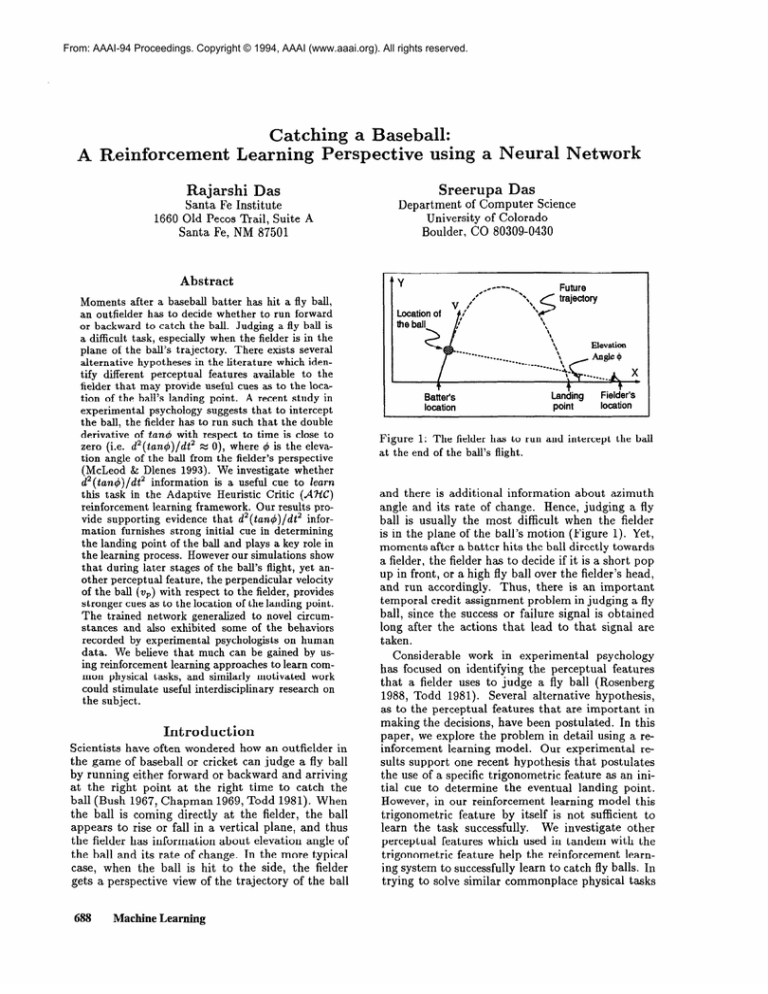
1: The fielder has to run and intercept
the ball
at the end of the ball’s flight.
and there is additional
information
about azimuth
angle and its rate of change.
Hence, judging
a fly
ball is usually the most difficult when the fielder
is in the plane of the ball’s motion (Figure 1). Yet,
moments after a batter hits the ball directly towards
a fielder, the fielder has to decide if it is a short pop
up in front, or a high fly ball over the fielder’s head,
and run accordingly.
Thus, there is an important
temporal
credit assignment
problem in judging a fly
ball, since the success or failure signal is obtained
long after the actions that lead to that signal are
taken.
Considerable
work in experimental
psychology
has focused on identifying
the perceptual
features
that a fielder uses to judge a fly ball (Rosenberg
1988, Todd 1981). Several alternative
hypothesis,
as to the perceptual
features that are important
in
making the decisions, have been postulated.
In this
paper, we explore the problem
in detail using a reinforcement
learning model.
Our experimental
resuits support
one recent hypothesis
that postulates
the use of a specific trigonometric
feature as an initial cue to determine
the eventual
landing
point,.
However, in our reinforcement
learning
model this
trigonometric
feature
by itself is not, sufficient, to
learn the task successfully.
We investigate
other
perceptual
features which used in tandem with the
trigonometric
feature help the reinforcement
learning system to successfully
learn to catch fly balls. In
trying to solve similar commonplace
physical tasks
Brancazio’s
I
m
Fielder at 99.5 m
6
Time (seconds)
Figure 2: The figure shows the variation in tan4 as
seen by three different fielders standing at 59.5 m, 79.5
The initial velocity
m, and 99.5 m from the batter.
of the ball is 30 m/s, directed at an angle 60’ from the
horizontal.
Here the range of the trajectory of the ball is
1
Symbol
@
ddldt
d2d/dt2
:D,dt
it,, ldt
Table
List of Perceptual
Features
to the Fielder
Available
Feature
Angle of Uevation
Rate of change of
Rate of change of
Distance between
Rate of change of
r
4
dg5/dt
ball and fielder
D (= -21,., the radial
velocity)
Velocity of ball perpendicular
to fielder
Rate of change of 21,
1: Brancazio
showed that,
with the possible
ex-
ception of d2q5/dt2,these features provide no significant
initial cue as to the location of the ball’s landing point.
Note that
D is inversely
proportional
to the apparent
size of the ball. Other possible perceptual
clude tunqb, d( tunqS)/dt, d2 ( tunb)/dt2.
features
in-
79.5 m, and since this simulation ignores -air resistance,
tan4 increases at a constant
rate only for the fielder
standing at 79.5 m.
using reinforcement
learning we not only learn more
about the reinforcement
learning models themselves
but also understand
the underlying
complexities
involved in a physical task.
The physics of judging
a fly ball
The problem of trajectory
interception
was analyzed
by Chapman
using Newton’s laws of motion (Chapman 1968). For a perfect parabolic
trajectory,
the
tangent of the ball’s elevation
angle 4 increases at a
steady rate with time (i.e. d(tan$)/dt
= constant)
over the entire duration
of flight, if the fielder stands
stationary
at the ball’s landing
point (Figure
2).
This simple principle holds true for any initial velocity and launch angle of the ball over a finite range.
If the ball is going to fall in front of the fielder,
then tanqi grows at first and then decreases
with
d2(tanq5)/dt2
< 0. On the other hand, if the ball
is going to fly over the fielder’s head, then tan4
grows at an increasing
rate with d2(tanqi)/dt2
> 0.
Chapman
suggested
that if a fielder runs with a constant velocity so that d(tanqi)/dt
is constant
then
the fielder can reach the proper spot to catch the
ball just as it arrives.
However, Chapman
neglected
the effects of aerodynamic drag on the ball which significantly
affects
the ball’s trajectory
and range.
When air resistance is taken into account,
Brancazio
claimed that
the specific trigonometric
feature cited by Chapman
cannot provide useful cues to the fielder (Brancazio
1985).
In addition,
Chapman’s
hypothesis
makes
the unrealistic
assumption
that the fielder runs with
a constant
velocity while attempting
to catch a fly
ball. Brancazio
went on to show that many of the
other perceptual
features
available to a fielder (see
Table 1) cannot provide significant
initial cue to determine
the landing point of the ball. After eliminating
several possible
candidate
features,
Brancazio hypothesized
that the angular acceleration
of
the ball d2qi/dt2 provides
the strongest
initial cue
as to the location of the eventual landing point. He
also conjectured
that the angular acceleration
of a
fielder’s head while the fielder tries to visually track
a fly ball, might be detected
by the vestibular
system in the inner ear, which in turn might provide
feedback
to influence the judgement
process of the
fielder.
Recent experimental
results obtained
by McLeod
and Dlenes
(McLeod
& Dlenes
1993) however
show that an experienced
fielder runs such that
d2(tanqh)/dt2
is maintained
close to zero until the
end of the ball’s flight.
McLeod and Dlenes suggest that this is a very robust strategy
for the real
world, since the outcome
is independent
of the effects of aerodynamic
drag on the ball’s trajectory,
or
the ball following a parabolic path. However little is
understood
about how human beings learn to intercept a free falling ball (Rosenberg
1988) and exactly
how d2(tam#)/dt2
information
helps in the learning
process.
In this paper, we provide supporting
evidence that
d2(tanqb)/dt2 information
furnishes strong initial cue
as to the landing point of the ball and plays a key
role in the learning process in a reinforcement
learning framework.
However, in the later stages of the
ball’s flight, d2(tan+)/dt2
provides
conflicting
cues
and the reinforcement
learning model has difficulty
in intercepting
fly balls. We delineate
the cause of
this problem
and use an additional
perceptual
feature that helps in learning the task.
Reinforcement Learning
689
Using reinforcement learning to catch
a baseball
We use Barto,
Sutton
and Anderson’s
Multilayer
Adaptive
Heuristic
Critic (AM) model (Anderson
1986) to learn the task. The general framework
of
reinforcement
learning is as follows: an agent seeks
to control a discrete time stochastic
dynamical
system. At each time step, the agent observes the current environmental
state x and executes
action Q.
The agent receives
a payoff (and/or
pays a cost)
which is a function
of state x and action a, and
the system makes a probabilistic
transition
to state
y. The agent’s goal is to determine
a control policy that maximizes
some objective
function.
d’)CC
is a reinforcement
algorithm
for discovering
an extended plan of actions which maximizes
the cumulative long-term
reward received
by an agent as a
result of its actions.
In the AEC framework,
the model consists of two
sub-modules
(networks);
one is the agent (action
network),
that tries to learn search heuristics
in the
form of a probabilistic
mapping
from the states to
the actions in order to maximize
the objective function. Typically
the objective
function
is a cumulative measure
of payoffs and costs over time.
The
other module is the critic (evaluation
network) that
tries to evaluate
the agent’s performance
based on
the reinforcement
received from the environment
as
a result of the action just taken.
In our implementation
of the d7fC model, the action u(t), taken by the agent (action network)
corresponds
to the instantaneous
acceleration
of the
fielder at time t. The state,
2, is assumed
to be
described
by a set of inputs provided
to the model
at every time step.
The action network generates
real valued actions, a(t), at every time step, similar
to that described
by Gullapalli
(Gullapalli
1993).
The output
of the action network
determines
the
mean, p(t), and the output
of the evaluation
network determines
the standard
deviation,
a(t) of the
acceleration,
u(t), at a particular
time.
P(t)
= output
of action
a(t) = max(r(t),
network,
0.0)
where r(t) is the output of the evaluation
network.
Assuming
a Gaussian
distribution
\E, the action a(t)
is computed
using p(t) and a(t).
In the course of learning,
both the evaluation
and
action networks
are adjusted
incrementally
in order
to perform
credit assignment
appropriately.
The
most popular
and best-understood
approach
to a
credit assignment
problem
is the temporal di$erence (TD) method
(Sutton
1988), and the AM
is a
TD based reinforcement
learning
approach
(Anderson 1986).
Since the objective
of learning is to maximize
the
agent’s performance,
a natural
measure
of performance is the discounted
cumulative
reinforcement
690
Machine Learning
(or for short,
utility)
(Barto
et al. 1990):
where r(t) is the discounted
cumulative
reinforcethe
ment (utility)
starting
from time t throughout
future, f(t) is the reinforcement
received after the
transition
from time t to t + 1, and 0 < 7 5 1 is
a discount
factor, which adjusts the importance
of
long term consequences
of actions.
Thus the utility,
r(t), of a state x is the immediate
payoff plus the
utility, r(t + l), of the next state y, discounted
by
y. Therefore
the desired function must satisfy:
r(t) = f(t) + yr(t + 1)
Relating these ideas to the d?fC model, the output
of the evaluation
network corresponds
to r(t). During learning, the evaluation
network tries to generate
the correct utility of a state. The difference between
the actual utility of a state and its predicted
utility
(called the TD error) is used to adjust the weights
of the evaluation
network using backpropagation
algorithm
(Rumelhart
et al. 1986). The action network is also adjusted
according
to the same TD error (Sutton 1988, Lin 1992). The objective
function
that determines
the weight update rules is defined
aS:
f(t)yr(t
+
Error
=
f(t)
- r(t)
+ 1) - r(t)
e while the ball
is in the air,
e if the ball has
hit the ground.
Simulation details
The perceptual
features
that are available
to the
fielder while judging a fly ball define the input variables of our system.
At any time t, the inputs to
the system include: 4, d2(tanq5)/dt2,
vf----the velocity of the fielder, and a binary flag which indicates
whether
the ball is spatially
in front of or behind
the fielder.
Thus the system receives no information about the absolute
coordinates
of the ball or
the fielder at any point in time. Initially, the fielder
is positioned
at a random distance in front of or behind the ball’s landing point.
The initial velocity
and the initial acceleration
of the fielder are both
set to zero. Once the ball is launched,
the fielder’s
movement
is controlled
by the output
u(t) of the
action network which determines
the fielder’s acceleration at time t. The simulation
is continued
(see
Appendix
for the equations)
until the ball’s trajectory is complete
and a failure signal is generated.
If the ball has hit the ground and the fielder has
failed to intercept
the ball, the failure signal f(t) is
proportional
to the fielder’s distance from the ball’s
landing point.
while the ball is in the air,
if D(fintaZ) 5 R (Success!),
if D(finuZ)
> 7Z (Failure!).
50
40
d
.&o
ai
P
%20
r
3
0
-1
-1 5 '
0
10
Fielder at 59 m Ball falls very close in front
1
Tin& (se&k)
\
4
1
1
I
5
0
0
la0
400
504
coil
700
800
wo'
106D
Cumulative numiber of trials
Figure 3: The variation of d2(tan4)/dt2
as seen from
three different positions. Aerodynamic drag is taken into
consideration
in this simulation, and for the same initial
parameters as in Figure 2, the range decreases to 57.5 m.
The ball touches the ground at t = 4.9 second. Note that
for the fielder stationed very close to the ball’s landing
point at 59 m, the d2(tand)/dt2
is close to zero for most
of the ball’s flight, but it increases dramatically
at the
end.
where D( f inal) is the distance between the ball and
the fielder when the ball hits the ground, R is the
catching
radius
and C is a positive
constant.
In
order to account for last moment adjustments
made
by the fielder (for example,
making a final dive at
the ball !), a catch is considered
successful if the ball
hits the ground within a region around the fielder’s
position
defined by the catching
radius, R. In our
simulations,
the catching
radius was set to 2 m. It
may be noted here that the information-whether
the
ball fell in front of or behind
the fielder-is
not a
part of the reinforcement
signal.
This information
is provided
as a part of the input signal and thus,
all throughout
the ball’s trajectory,
the fielder knows
whether
the ball is in front of or behind the fielder.
The inputs
to the network
are computed
as follows.
The raw inputs,
as determined
by the system dynamics
(defined
in the Appendix),
are first
clipped using the following lower and upper bounds
(indicated
by 0): (-10.0, lO.O)m/s for the fielder’s
for the fielder’s accelvelocity, v~f; (-5.0, 5.0)m/s2
eration;
(O*, lSO*) for 4; (-25.0,25.0)m/s
for zlP
(referred
to in the next section);
(-0.5,0.5)sV2
for
d2(tunr$)/dt2.
The clipped inputs are then normalized between 0.0 and 1.0 and finally presented
to the
network.
Nevertheless,
while determining
the system dynamics
none of the values are either scaled
or clipped.
A sampling
frequency
of 10 Hz (i.e.
At = 0.1s) is used during the simulation
of the system.
Results
Our results, using
that d2(tun+)/dt2
the AXC learning approach,
show
information
by itself is not suffi-
Figure 4: The plots show the number of successful
catches every 50 trials as a function of total number
of trials for three different sets of input features.
The
three sets of features are (A) both d2(tan4)/dt2
and vP.
(B) d2(tan4)/dt2
but not up, (C) d2(4)/dt2.
(The other
input features: 4, VU~
and the binary flag were used in all
three sets). The initial angle of the ba.ll is chosen randomly between [50°, 700]. The fielder’s initial position is
also chosen from a random distribution
between [47.5m,
67.5m].
The initial velocity and initial acceleration of
the fielder are both set to zero in every trial.
cient to learn the task at hand.
After an initial
learning
period,
the system
surprisingly
learns to
move the fielder away from the ball’s landing point
instead of moving towards
it. Figure 3 delineates
the underlying
problem.
For a fielder standing
at
the ball’s landing point, d2(tun4)/dt2
is always zero.
However, if the fielder is only a small distance
away
is close
from the ball’s landing point, d2(tun+)/dt2
to zero for most of the ball’s flight, until near the
end when it increases dramatically.
Thus large and
small magnitudes
of d2(tun$)/dt2
can be associated
with both large and small values of negative
failure signals providing
conflicting
cues to a learning
system.
We therefore
investigate
other perceptual
features that might help in the learning
process by
removing the ambiguity.
Figure 4 plots the performance
of the network
when different
sets of inputs (perceptual
features)
are used (in addition to 4, vf, and the binary direction flag). In the figure, each learning
curve is an
average of 10 independent
trials, where each curve
corresponds
to one of the three different sets of perceptual features (A) d2(tan4)/dt2 and up, where vup
is the perpendicular
component
of the ball’s velocity as seen by the fielder, (B) d2(tun+)/dt2
LMcLeod
& Dlenes’ hypothesis),
and (C) d2($)/dt
(Brancazio’s hypothesis).
In the simulations
each trial
begins with the fielder at a random position in the
range [47.5m, 67.51 in front of the ball and the ball
is thrown with an initial angle randomly
distributed
in [50°, 70’1. The plots show that the network could
not learn the task using only d2(tun$)/dt2
or using
Reinforcement Learning
691
Fielder at 59 m
Ball falls very close
in front
Fielder at 89 m
Ball drops in front
1
Figure 5: The variation of the perpendicular
component of the ball’s velocity as seen from three different
positions. The initial parameters are the same as in Figure 2. The ball touches the ground at t = 4.9 seconds.
Note that the three plots are very close to each other for
the first three seconds, and diverge only at the end of
the ball’s flight.
only d2($)/dt2. Let us analyze why up could possibly help in learning (Brancazio
1985). Figure 5 plots
the variation
of up as seen by the fielder standing
at
three different positions.
Initially,
up provides little
cue as to the balls landing point, but as the ball’s
flight comes to an end, vP is significantly
different
for the fielders standing
at different
positions.
Interestingly
enough, the network is able to learn the
task, since vP information
adds the necessary
discriminating
ability in judging
fly balls during the
latter stages of the ball’s flight.
The above results suggests
that in our reinforcement learning
model both d2(tun4)/dt2
and vP are
necessary
for learning
the task of catching
a ball.
During the initial part of the ball’s flight, the system
learns to keep d2(tunqS)/dt2 very small, and move in
the correct direction.
Towards the end of the ball’s
flight, when d2(tun4)/dt2
increases
drastically,
the
to run
system
learns to use vP to decide whether
forward or backward.
Figure 6 shows space-time
plots of the fielder’s
trajectories
before and after training
for 20 different trials (the initial positions
of the fielder are set
randomly,
although
the initial angle of the ball is
identical
in each trial).
In their experiments
with
a skillful fielder, McLeod and Dlenes observed
that
the fielder does not automatically
run to the point
where the ball will fall and then wait for it, rather
the fielder tracks the ball throughout
its trajectory
till it hits the ground.
We see a similar behavior
in Figure 6 after the system has learned
to catch.
More interestingly,
Figure 6 shows that a fielder who
is initially positioned
slightly in front of the landing
point of the ball, goes through
a temporary
phase
when the fielder actually runs away from the eventual landing point of the ball. The data presented
692
Machine Learning
Tim: (sec&
4
5
After lraining -
Figure 6: The two space-time plots show the fielder’s
distance from the -batter in 20 trials, before (left) and
after (right) training for 10000 trials. The initial parameters of the baJl are the same as in Figure 2 and
the fielder’s initial position is chosen from a random distribution [47.5m, 67.5m]. The initial velocity and the
initial acceleration of the fielder are both set to zero in
every trial. The ball’s range is 57.5 m which is reached
at t = 4.9 second.
by McLeod and Dlenes shows surprisingly
similar
behavior
among experienced
fielders.
Our last set of simulations
focus on the generalizational performance
of a trained network.
Figure 7
depicts the results. The network is first trained with
trials where the initial angle of the ball is randomly
set to a value in the range [57”, 62O]. After training,
we test the network on trials where the initial angle
is randomly
selected from increasing
ranges:
from
[57’, 62’1 to [45’, 75’1. As is evident from the plot,
the network is able to generalize and perform reasonably well in situations
which it had not experienced
during the training
phase.
Note that the range of
ball’s trajectory
during training is bounded between
56.lm (for 57”) and 62.3m (for 62”) which is much
smaller than the range of the ball’s trajectory
during
testing (which varies between 69.69m (for 45”) and
34.36m (for 75O)). Th ese results in generalization
performance
indicate that the network is able to extract important
rules from the perceptual
features
is the aerodynamic
drag force constant
equal to
m-l
for a baseball (Brancazio
1985). Using a sampling
time of At second,
the above equaK
0.005249
tions are numerically
tives as follows:
Ax
= v,At
integrated
(2)
+ 0.5y”(At)2
+ 0.1667y”‘(At)3,
(3)
and 21’
= (&X1’
+ q, y”)/v.
are also updated
FLS:
t&red
Average
7:
network
generalization
is shown.
The
performance
network
of a
is trained
on
trajectories
with the ball’s initial angle ranging between
57O - 62O. The trained network is then tested on trials where the initial angle ranged between 45O - 75O.
The simulations
are averaged over 10 runs with the
fielder’s initial position chosen from a random distribu-
Given the
ball, and
calculate
including
tions and
than
memorize
Conclusion
The
goal
inforcement
of this
the training
and future work
research
learning
data.
model
is to
determine
can learn
balls using a specific-trigonometric
if a re-
to catch
feature
fly
suggested
in the experimental
psychology
literature.
We have
shown that for the reinforcement
learning model discussed in this paper, d2(tand)/dt2
and&
information -play- a vital-role
in the learning
the task.
It
is possible
that in later stages of the ball’s trajectory, an experienced
fielder might use other perceptual features
like stereoscopic
vision as the guiding
mechanism.
We are currently
investigating-such
a
hypothesis.
We believe much can be gained by using reinforcement
learning approaches
to learn common physical
tasks,
and we hope that this work
would stimulate
useful interdisciplinary
research on
the subject.
Acknowledgements
We thank C. W. Anderson,
K. L. Markey, M.C.
Mozer, S.J. Nowlan, and the anonymous
reviewers
of this paper for their valuable suggestions.
Appendix:
The Equations
The equations
of motion
projectile
can be expressed
2” = -Kvv3:,
in two
as:
of Motion
dimensions
y” = -Kvvy
- g
for a
(1)
where 2” and y” are the instantaneous
horizontal
and vertical
accelerations,
v, and vY are the horizontal and vertical
components
of the velocity of
the ball v, g is the acceleration
due to gravity and
y”’ = -K(v’vy+vy”),
The velocity
components
Au,
= /‘(At)
+ 0.5z”‘(At)2,
(4)
Au,
= /‘(At)
+ 0.5y”‘(At)2
(5)
current coordinates
of the fielder and the
their respective
velocities,
i t is possible to
the variables associated
with 4, and tan4
their derivatives
using trigonometric
equacalculus.
References
tion [47.5m, 67.5m].
rather
deriva-
+ 0.1667x”‘(At)3,
where z”’ = -K(v’v~+vz”),
Figure
third
+ 0.5;c”(At)2
Ay = vyAt
Range of Initial Launch Angle (in degrees)
using
Anderson,
C.W.
1986. Learning and Problem Solving with multilayer connectionist
systems.
Ph.D. diss.,
Computer Science, Univ. of Massachusetts,
Amherst.
A.G.,
Sutton,
R.S., & Watkins,
C.J.C.H.
Barto.
1990.
“Learning and sequential decision making,,, In:
M. Gabriel & J.W. Moores (Eds.), Learning and computational neuroscience,
MIT Press.
“Looking into Chapman’s
Brancazio,
P.J. 1985.
homer:
The physics of judging a fly ball,” American
Journal of Physics, Vol. 53, No. 9, pp. 849-855.
Bush, V. 1967. Science is not enough, Wm. Morrow
Co., NY.
Chapman,
C. 1968. “Catching a baseball,” American
Journal of Physics, Vol. 36, No. 10, pp. 868-870.
Gullapalli,
V. 1990. “A stochastic reinforcement learning algorithm for learning real-valued functions,” Neural
Networks, Vol. 3, pp. 671-691.
Lin, L.J. 1992. “Self-improving reactive agents based
on reinforcement learning, planning, and teaching,” Machine Learning, 8, pp. 293-321.
McLeod,
P. & Dlenes,
Z. 1993. “Running to catch
the ball,” Nature, Vol. 362, pp. 23.
Rosenberg,
K.S. 1988. “Role of visual information in
ball catching,”
Journal of Motor Behavior,
Vol. 20, No.
2, pp. 150-164.
Rumelhart,
D.E., Hinton, G.E., & William,
R.J.
1986. “Learning internal representations
by error propagation,> Parallel
Distributed
Processing:
Explorations
in the microstructure
of cognition.
Vol. 1., Bradford
Books/MIT
Press.
Sutton. B.S. 1988. “Learning to predict by the methods of temporal differences.”
Machine Learning,
3, pp.
9-44.
Todd, J.T. 1981. “Visual information about moving
objects,,’ Journal of Experimental
Psychology:
Human
Perception
810.
and Performance,
Vol.
7, No.
4, pp.
Reinforcement Learning
7%
693