From: AAAI-91 Proceedings. Copyright ©1991, AAAI (www.aaai.org). All rights reserved.
noses
Johan
de Kleer
Xerox
Palo Alto Research Center
3333 Coyote Hill Road, Palo Alto CA 94304 USA
Email: dekleer@xerox.com
Abstract
Model-based
diagnosis is based on first-principles
reasoning using the behavioral
specifications
of the
primitive components
of a device. Unless the computational
architecture
of the model-based
reasoning engine is carefully designed, combinatorial
explosion renders the approach useless for devices consisting of more than a handful of components.
This
paper analyzes the diverse origins of this combina
torial explosion and outlines strategies to cope with
each one. The resulting computational
architecture
for model-based
diagnosis provides orders of magnitude performance
improvement
on large examples,
making model-based
approach practical for devices
consisting of on the order of 3000 components.
1
Introduction
Model-based
diagnosis [2] is a very general approach for
diagnosing devices from first principles alone. The GDE
[6] and Sherlock [7] s y s t ems provide an ATMS-based
[3],
computational
framework for diagnosing multiple faults.
Unfortunately,
the computational
complexity of the algorithms makes them impractical
to use for most devices
consisting of more than a few dozen components.
This
paper presents a technique for focusing the processing of
these diagnostic engines and the underlying
ATMS. By
exploiting these techniques
both GDE and Sherlock become orders of magnitude
more efficient and can easily
diagnose devices which were inconceivable
to even consider before. For example, they can now diagnose many
circuits of over 3000 components
in less than a minute of
CPU time on a Symbolics XL1200, while without these
techniques
the same machine runs out of memory in a
few hours on the same task. The techniques
described
in this paper are general and should easily extend to
other approaches
to model-based
diagnosis [12; 14; 15;
18; 191. The techniques
can also be generalized to apply
to most-probable-first
search in general - although this
topic is outside of the scope of this paper.
Our techniques
are based on two fundamental
intuitions.
The first is to precisely focus the diagnostic
reasoning
to those sections of the device in which the
fault(s) probably lie and to ignore the other parts of the
device. The second is to recognize that it is sufficient
842
DIAGNOSIS
to identify the most probable
proximate
their probabilities.
necessary to find all minimal
2
diagnoses and to only apIn particular,
it is rarely
diagnoses.
Example
The intuitions
can be illustrated
with the faulty n-bit
adder illustrated
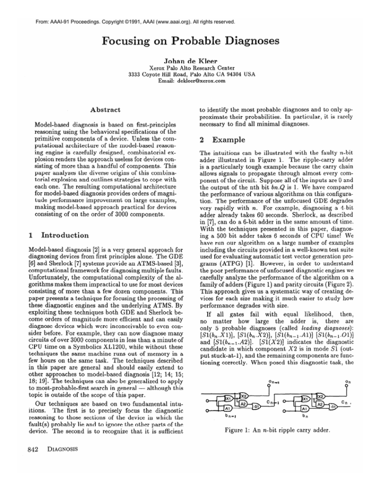
in Figure 1. The ripple-carry
adder
is a particularly
tough example because the carry chain
allows signals to propagate
through almost every component of the circuit. Suppose all of the inputs are 0 and
the output of the nth bit bn.Q is 1. We have compared
the performance
of various algorithms on this configuration. The performance
of the unfocused GDE degrades
a 4-bit
very rapidly with n. For example, diagnosing
adder already takes 60 seconds.
Sherlock, as described
in [7], can do a 6-bit adder in the same amount of time.
With the techniques
presented
in this paper, diagnosing a 500 bit adder takes 6 seconds of CPU time! We
have run our algorithm
on a large number of examples
including the circuits provided in a well-known test suite
used for evaluating automatic
test vector generation programs (ATPG)
[l]. H owever, in order to understand
the poor performance
of unfocused diagnostic engines we
carefully analyze the performance
of the algorithm on a
family of adders (Figure 1) and parity circuits (Figure 2).
This approach gives us a systematic
way of creating devices for each size making it much easier to study how
performance
degrades with size.
If all gates
fail with
equal
likelihood,
then,
there
are
no matter
how large
the
adder
is,
only 5 probable
diagnoses
(called leading diagnoses):
[Sl(b,.Xl)],
[Sl(b,.X2)],
[Sl(b,-I.A1)]
[Sl(b,-l.Ol)]
and [Sl(b,-l.A2)].
[Sl(X2)]
indicates
the diagnostic
candidate
in which component
X2 is in mode Sl (output stuck-at-l),
and the remaining components
are functioning correctly.
When posed this diagnostic task, the
Qn.4
on
bn-1
Figure
bn
1: An n-bit
ripple
carry adder.
modeled by one good mode (G) and three faulty modes:
output stuck-at-l
(Sl), output stuck-at-0
(SO) and unknown (U). (0 ur analysis here focuses on Sherlock because it subsumes GDE.)
0
rutb.-r
Figure 2: A 3-bit parity
n bit parity circuit.
circuit
is cascaded
to obtain
an
focused Sherlock finds exactly these 5 diagnoses for any
n. Moreover,
it requires only 7 minimal conflicts (for
all n > 1). In contrast,
with the unfocused
GDE the
number of conflicts grows rapidly with n (e.g., at n = 8
there are 1545 conflicts).
Also the CPU time taken to
find these 5 diagnoses grows very slowly with n (see Figure 5).
Computationally
the techniques of this paper operate
by simultaneously
limiting the execution of consumers
(i.e., the propagation
of values through the constraints
modeling the components),
restricting
the ATMS label
update
algorithms,
and controlling
candidate
generation. Ideas for controlling
the execution
of consumers
are discussed in [5; 6; 111. Controlling
the ATMS itself is discussed in [9; 10; 111. The unique contribution
of this paper is the monolithic
most-probable-first
diagnostic strategy that fits these pieces together in a novel
combination
to obtain vastly superior performance
on
diagnostic tasks.
3
The source
of the explosion
GDE’s and Sherlock’s
three processing phases.
Prediction:
diagnostic
Use the observations
els to make predictions.
process
consists
and component
of
mod-
Conflict
recognition:
Recognize
discrepancies
between predictions
and observations
to construct a set
of conflicts, that is, sets of component
modes which
cannot all hold simultaneously.
Candidate
generation:
Identify
assignments of modes to all the components
which explain
all the symptoms,
that is, not containing
any conflicts
as subsets. These are the diagnoses.
In GDE and Sherlock this process is performed incrementally in response to every new observation.
Nevertheless for each new observation
these three steps are
performed sequentially.
In diagnosing a large device, each of these three steps
exhibits a combinatorial
explosion.
We analyze a family of different size adders (see Figure 1). Each gate is
The prediction phase is supported
by the ATMS and
Each prediction
consists of
its consumer architecture.
a specific value for a device variable and a (consistent)
conjunction
of underlying
assumptions
(called an environment) which, together with the observations,
imply
that value. In all of our examples each assumption
is a
behavioral
mode of some component,
although this restriction is not necessary in general (for example, in [16]
assumptions
are used to represent time and modeling assumptions).
If all the inputs are 0, then the predictions
for b0.Q = 1 are:
Sl(bO.X2)
G(bO.X2)
3 b0.Q = 1,
A Sl(bO.Xl)
+ b0.Q = -1.
For example,
the second prediction
states that if the
exclusive-or gate X2 of bit 0 is operating
correctly and
the exclusive-or gate Xl has its output stuck at 1, then
E --) n predicthe output bit of bit 0 is 1. A prediction
tion is minimal if there is no other prediction
E’ + n
such that E’ c E. The prediction
phase finds all minimal predictions.
As every subset of assumptions
can lead to a distinct
prediction
there are typically an exponential
number of
possible predictions.
The ATMS exploits the monotonicity property that if a fact follows from a set of assumptions it follows from every superset as well. Hence, it
is only necessary to compute and represent the minimal
environments
(under subset) for each fact. These are
the minimal predictions.
Although considering only the
minimal predictions leads to great improvements,
we see
from the data that we do not escape the combinatorial
explosion.
Figure 3 plots the total number of minimal
predictions
for all circuit variables vs. the number of
gates in the ripple carry adder.
This growth curve is
typical for the circuits we have looked at.
The next phase of the conventional
model-based
algorithm, conflict recognition,
suffers from the same combinatorial
growth as prediction.
A conflict is an environment which is inconsistent
with the observations.
In
analogy with prediction,
we are only interested
in the
minimal conflicts.
Consider the case where we observe
the symptom bn.Q = 1 (bn.Q should be 0 because all the
adder inputs are 0). Figure 4 plots the the number of
minimal conflicts vs. the number of gates in the ripple
carry adder.
The candidate
generation
phase often exhibits combinatorial
growth as well.
Almost by definition,
the
number of diagnoses grows exponentially
in the number
of components.
Therefore most earlier approaches to
model-based
diagnosis find minimal diagnoses. The notion of minimal diagnosis is easily extended to the case
where there are fault modes and produces significant
savings. Intuitively
we say a diagnosis is non-minimal
if
DE KLEER
843
we can replace any faulty mode with a good mode and
still have a diagnosis, or if we can replace the faulty U
mode with any other mode and still be a diagnosis.
If
U is the only fault mode, then this definition is identical
to the usual one of minimal diagnosis.
Although devices may have exponentially
many minimal diagnoses, this exponential
is often avoided in practice.
For example,
the n-bit adder has 3n - 1 minimal diagnoses.
Of course, this is still not of much help,
as 74 minimal diagnoses for a 25-bit ripple carry adder
is unreasonable.
All but five of these 74 diagnoses are
extremely unlikely multiple faults which should not be
considered until the more likely (single) faults are eliminated.
We saw earlier that if a bit position is symptomatic, then no matter how many bits wide the adder
is, there are only five probable diagnoses after observing
that bn.Q = 1.
60
# of components
Figure
gates.
3: Number
of minimal
predictions
vs. number
of
The computational
observations
of this section are
predicated
on using multiple faulty behavior modes for
If we were to use the GDE-style
models
components.
which did not characterize faulty behaviors, then the results would be less explosive.
The number of minimal
diagnoses vs. circuit size is identical; the plot of predictions vs. circuit size becomes polynomial
and the the
plot of conflicts vs. circuit size becomes linear.
Nevertheless, even a linear number of minimal diagnoses is
still unacceptable
for our example.
The results of this
paper thus provide significant
computational
advantage
to both GDE-style and Sherlock-style
diagnoses.
4
Focusing
We briefly describe a computational
architecture
for
reining in the combinatorial
explosion of all three phases
of model-based
diagnosis. The conventional
architecture
requires first completing prediction,
then conflict recognition, and finally candidate generation.
Within our new
architecture
all three processes are intermixed
so that
the computational
effort expended
in prediction,
conflict recognition and candidate generation are simultaneously minimized.
Rather than generating
all candidates
at once, at the very end - we generate the candidates
one at a time (based on the known conflicts), and then
focus prediction and conflict recognition
only on testing
the consistency
of the single candidate
with respect to
new observations.
20
30
40
50
# of components
Figure
gates.
844
4: Number
DIAGNOSIS
of minimal
conflicts
vs.
number
of
Candidates
are generated in decreasing order of probability, thus candidate
generation
can be cut off once
all the probable
candidates
have been enumerated
little effort is expended
on the overwhelmingly
larger
set of improbable
diagnoses.
Note that this presents a
bootstrapping
problem: generating the candidates in the
proper order requires knowing their posterior probabilities. These probabilities
are computed
from the predictions and conflicts that follow from each candidate.
Computing
these predictions
and conflicts for all candidates would defeat the purpose of the focusing mechanism - since the whole point is to only compute them
for the most probable candidates.
To solve this “chicken
and egg” problem we generate candidates
one at a time
using the prior probabilities
as an estimate of their posterior probabilities.
We then perform prediction
and
conflict recognition
on each candidate
individually.
Finally the strategy estimates
the posterior probabilities
and the ordering of these candidates
based on the information gained. Our experience is that these prior probabilities provide a reasonably
accurate estimate, and that
only a small amount of effort is wasted pursuing candidates that turn out to be improbable.
Once the probable candidates
are generated, probe points are proposed
that best distinguish
among these candidates.
4.1 Focusing
candidate
generation
The driving intuition
behind our framework is to focus
the reasoning on what will ultimately
be the most probable diagnoses.
Instead of estimating
the probabilities
in some post-processing
stage we exploit and incorporate the probabilities
from the beginning.
The candidate
generator
does most-probable-first
search.
Like GDE
and Sherlock we determine the posterior probabilities
of
candidates
by Bayes rule:
P(GlXi
= Qk:) =
The prior probability
assuming independence
P(Xi = Gk IG)P(G)
=
of behavior
component
Conflict
candidates
recognition
is necessary to determine
which
are eliminated
by the observations,
i.e., when
is necessary to determine
P(Xi = ~iklC?) = 0. Prediction
which candidates
are supported
by the evidence, i.e.,
when p(xa = v~kjCi> = 1. The objective of our framework is to correctly identify the probability
ranking of
each diagnosis, but not necessarily establish its absolute
probability.
Therefore,
the denominator
p(xi = vik) is
just a normalization
and does not need to be accurately
determined
to rank candidates.
From Bayes rule we know that the posterior
ity of any candidate
is bounded above by:
P(GlXi
= Gk) I
propagation
The original GDE unfocused engine using a conventional ATMS finds all minimal predictions
and conflicts
regardless of leading candidates.
Our focused algorithm
uses the tentative candidates
generated by the best-first
search to focus its inferences.
For each tentative candidate, the HTMS constructs
at most one prediction for
each circuit quantity and (usually) at most one conflict.
This avoids the exponential
explosion we see in Figure 3,
but critically relies on a method to generate the tentative
leading candidates.
hen to stop
generating
candidates
-
p(m) mECl
where p(m) denotes the prior probability
mode m being manifested
(i.e., a particular
being in a particular
mode).
constraint
Our co-routining
candidate
generator provides the next
most probable candidate
based solely on its prior (and
the conflicts which have been accumulated
thus far). We
must perform sufficient reasoning on this candidate
to
correctly establish its posterior probability.
In order to
do so efficiently we must perform prediction
and conflict recognition
focused on this candidate
alone.
Instead of using a conventional
ATMS we use a hybrid
TMS (HTMS [9]) which h as some of the properties of a
focused ATMS and some of the properties of a conventional TMS.
5
P(Xi = WC)
of any candidate
Cl is evaluated
of component
failures:
P(G)
Focusing
4.2
probabil-
PW
P(Xi = w)
We have incorporated
this formula directly into the candidate generator.
Our candidate
generator
performs a
co-routining
best-first search. The candidate
generator
returns exactly one candidate
at a time. It returns the
next most probable candidate
based on its prior probability. In addition, the candidate generator avoids candidates subsumed by conflicts that have been encountered
thus far.
Our best-first
search is guaranteed
to generate candidates in decreasing order of their prior probabilities.
If
all the leading diagnoses predict the same observations,
then we see from Bayes rule that the candidate generator
will find candidates in decreasing order of their posterior
probabilities.
Candidate
generation
stops when one of
the following criteria is met.
1. The best candidate
has posterior (estimated)
probability greater than Ica (we usually use ka = 100) times
the prior probability
of the next candidate
to be returned by the candidate generator.
2. There are ICI > 1 or more candidates.
As the overall
task usually requires probing, its is often preferable to
avoid generating
all leading candidates
because many
of them will be eliminated
by the next probe anyway.
Usually a good probe can be selected using just a few
of the candidates.
3. The
sum of the probabilities
all the candidates
exceeds more than k3 (usually ka = .75) of the probability mass of all the candidates.
We approximate
this
latter probability
mass by setting to total mass to 1
initially and subtracting
from this the probability
of
every explicitly eliminated
candidate.
If diagnoses do not all predict the same observations
(this usually occurs when U modes appear in diagnoses),
then the relative priors do not establish
the relative
posteriors.
Therefore,
our architecture
maintains
two
lists of candidates
ordered by their (estimated)
posterior probabilities.
The first list II contains all candidates
whose posterior probability
is guaranteed
to be greater
DE KLEER
845
than the prior of the next candidate
which the candidate generator will provide. The second list 12 contains
candidates
whose posterior probability
is currently less
than the next candidate
the candidate
generator
provides. Thus, during the best-first search, even though no
new candidates
may be found by the search, candidates
may be moved from 12 to II. The list Zr is considered
the list of leading diagnoses or candidates
- 12 is not
used in the stopping criteria.
The full paper describes
some strategies to better estimate posterior probabilities
during search and thus prevent Z2 from becoming large.
These are useful primarily in cases where there are multiple U modes and where outputs are measured before
inputs, and were not used in any of the examples of this
paper.
# of components
6
Proposing
a new probe
Figure 5: Running time in seconds
an adder) on an XL1200
If II contains multiple, differentiable
diagnoses, then additional probes need to be made to identify the correct
diagnosis. The minimum entropy technique of GDE can
be applied without modification
using II as the set of
diagnoses.
The minimum
entropy technique is an algorithm based on the presupposition
that there are a very
large number of diagnoses such that multistep
lookahead is unacceptably
expensive.
In our case there are
usually only a handful of leading diagnoses and therefore we simply perform full lookahead (where the costs
at the leaves of the decision tree are the logarithm of the
current posterior probability
of the candidate).
Notice that it is unnecessary
to have a distinct test to
determine
whether the diagnoses in Zr are distinguishable. If they are not differentiable,
then we find no useful
probes. In that case, the diagnosis session is complete.
Using the our focused diagnostic engine produces the
same leading diagnoses as the unfocused engine but orders of magnitude
more efficiently.
The only serious
penalty incurred by using focusing is that it can propose suboptimal
probes.
The more diagnoses that are
available, the more accurately
hypothetical
probes can
be evaluated.
Without
additional
heuristics,
the probing strategy often proposes what intuition would say are
suboptimal
probes.
This occurs because every component which is not faulted in some leading diagnosis is essentially considered unfaulted.
As a consequence probes
distant from the actually possibly faulty components
are
often proposed (see [9]). This is suboptimal
for two reasons. First, as diagnosis proceeds and candidates
are
eliminated
this probe may be shown to be suboptimal.
Second, this generates
large conflicts.
Therefore,
our
implementation
has a simple heuristic which says that if
two probes have equal diagnostic
value, then pick that
probe point which is nearest a possibly faulty component.
846
DIAGNOSIS
7
vs. size in gates (of
Results
The focused diagnostic architecture
outlined in this paper improves the performance
of model-based
diagnosis
by orders of magnitude.
We can now diagnose devices
which were impossible
to analyze before.
To simplify
the explanations,
this data was obtained by setting the
probabilities
of the Sl and SO modes low and equal but
higher than that of the 27 modes. Comparable
results
should be obtained with any reasonable initial probabilities. The diagnostic
task for the adder is the same as
in the introduction.
The diagnostic task for the parity
is an input of all O’s and an erroneous output parity.
Our unfocused implementation
exceeds 60 seconds (on
a Symbolics XL1200) at approximately
50 components
(a 10 bit adder). F i g ure 5 shows that the running time is
roughly linear until about 1500 components
after which
performance
begins to degrade. Performance
monitoring
shows that this non-linear
degradation
is attributable
to
our implementation
of best-first search.
Although
the n-bit adder has 3n - 1 minimal diagnoses, our algorithm
identifies 5 leading diagnoses for
each n. For the parity circuit on the other hand the
number of leading diagnoses grows slowly with n (always n is the number of input bits).
The following table compares the number of minimal
predictions
with and without focusing. Column ‘G’ lists
the number of gates in the device. Parity’s results come
in groups of three because the circuit is constructed
in
multiples of 3.
algorithms.
It completely subsumes our previous algorithms and it is now being used in other research in
diagnosis [13; 161.
We are continuing
to analyze the algorithm with the
goal of improving
its overall performance.
Our experience raises some questions and open issues. The averages
in the tables obscure the fact that the algorithm does
surprisingly
poorly for certain symptoms (the unfocused
algorithm does even more poorly). If the circuit contains
a great deal of reconvergent
fanout, a significant amount
of redundancy,
and the particular
input vector and fault
cause these to be manifest, then the algorithm performs
relatively poorly. We also used a fault simulator to identify which faults were consistent with the symptoms.
In
somes cases, particularly
in ~7552, this strategy outperforms our algorithm.
If the sole goal were the identification of single-fault
diagnoses, then probably the most
efficient overall algorithm would be to use to the focused
diagnostic engine to find the first few conflicts, and then
switch to a conventional
simulator
to test the remaining single fault candidates.
Of course, such simulators
do not directly extend to multiple faults, probabilities,
minimum
entropy techniques,
explanations,
non-digital
devices, etc.
The following table compares the number of conflicts
with and without using our focused diagnostic architecture.
Adder conflicts
Parity conflicts
No focus
Focus
n
G
No focus
FOCUS G
1
5
3
3
0
0
0
In the case of the adder we see that the number of conflicts with focusing is constant in the size of the circuit.
In parity the number of minimal
conflicts grows very
slowly. The two tables show that for both circuits the
performance
improvement
is dramatic.
We ran the diagnostic algorithm on a variety of circuits from a standard
test suite of circuits [l]. We repeatedly
inserted a random fault in each circuit, found a sensitive input vector,
and applied our diagnostic engine to find the diagnoses.
The tables show the average number of minimal predictions (P) and minimal conflicts (c). The complexity of
our algorithm
is roughly proportional
to the number of
minimal conflicts it finds. Nevertheless,
for crude comparison purposes we include the current running times
as well. The unfocused
GDE results are not included
because it is much to slow to diagnose most of these
circuits.
circuit
A500
type
Adder
G
5000
As circuit ~7552 provoked so many of the cases of poor
performance,
we monitored
the performance
of the algorithm on it extensively.
We determined
that most of the
time was spent waiting for the disk to page in HTMS
data structures.
The working set of the algorithm significantly exceeded the amount of real memory available (6
MW). We are currently studying algorithmic
variations
to reduce the working set requirements
of the algorithm.
9
Acknowledgments
I thank Brian C. Williams
with whom I started this
work. Discussions with Daniel G. Bobrow, David Goldstone, Olivier Raiman,
Mark Shirley and Peter Struss
helped clarify the ideas and presentation,
7
i?
f
6537
7
6
References
[l] Brglez, F., and H. Fujiwara,
A neutral netlist of
10 combinational
benchmark
circuits and a target translator
in FORTRAN,
distributed
on a tape
to participants
of the Special Session on ATPG
on Circuits
and Fault Simulation,
Int. Symposium
and Systems, June 1985; partially characterized
in
F. Brglez, P. Pownall, and R. Hum, Accelerated
ATPG and fault grading via testability
analysis,
Proc. IEEE
tems, (June,
8
iscussion
The performance
of the new focused
rithm is dramatically
better than that
diagnostic
algoof the unfocused
Int. Symposium
on Circuits
and Sys-
1985) 695-698.
[2] Davis, R., and Hamscher, W., Model-based reasoning: Troubleshooting,
in Exploring artificial intelligence, edited by H.E. Shrobe and the American Association for Artificial Intelligence,
(Morgan Kaufman, 1988), 297-346.
DE KLEER
847
truth mainte[3] de Kleer, J., An assumption-based
nance system, Artificial InteZZigence 28 (1986) 127162. Also in Readings in NonMonotonic
Reasoning,
edited by Matthew L. Ginsberg, (Morgan Kaufman,
1987)) 280-297.
[4] de Kleer, J., Extending
the ATMS, Artificial InteZZigence 28 (1986) 163-196.
[5] de Kleer, J., Problem solving with the ATMS, Artificial Inteldigence 28 (1986) 197-224.
[6] de Kleer, J. and Williams,
B.C., Diagnosing
multiple faults, Artificial InteZZigence 32 (1987) 97130. Also in Readings in NonMonotonic
Reasoning,
edited by Matthew L. Ginsberg, (Morgan Kaufman,
1987)) 372-388.
[7] de Kleer, J. and Williams, B.C., Diagnosis with behavioral modes, in: Proceedings IJCAI-89,
Detroit,
MI (1989) 104-109.
[S] de Kleer, J., Using crude probability
estimates
to
Artificiad InteZZigence 45 (1990)
guide diagnosis,
381-391.
[9] de Kleer, J ., A hybrid TMS, submitted
for publication, 1990.
[lo] Dressler, O., and Farquhar,
A., Focusing ATMSbased problem solvers, Siemens Report INF-ZARM
13, 1989.
[ll] Forbus, K.D., de Kleer, J ., Focusing the ATMS,
Proceedings
AAAI-88,
Saint Paul, MN (August
1988), 193-198.
[12] Genesereth,
M.R., The use of design descriptions
in automated
diagnosis,
Artificial Intedligence 24
(1984) 411-436.
[13] Goldstone,
D.J ., Managing
bookkeeping
for ana
log diagnosis, Proceedings AAAI-91, Anaheim, CA,
(August, 1991).
[14] Hamscher,
W.C., Model-based
troubleshooting
of
digital systems,
Artificial Intelligence
Laboratory,
TR-1074, Cambridge:
M.I.T., 1988.
[15] Raiman, O., Diagnosis as a trial: The alibi principle, IBM Scientific Center, 1989.
[16] Raiman,
O., de Kleer, J ., Shirley,
M.H., and
Saraswat,
V., Characterizing
Non-Intermittency,
Proceedings
AAAI-91,
Anaheim,
CA, (August,
1991).
[17] Shirley, M.H., Generating Tests By Expdoiting DePhD thesis, MIT, January 1989.
signed Behavior.
[18] Struss, P., Extensions
to ATMS-based
Diagnosis,
in: J.S. Gero (ed.), Artificial
Intelligence
in Engineering:
Diagnosis and Learning,
Southampton,
1988.
[lQ] Struss, P., and Dressler, O., “Physical negation” Integrating
fault models into the general diagnostic engine, in: Proceedings IJCAI-89
Detroit, MI
(1989) 1318-1323.
848
DIAGNOSIS