From: AAAI-88 Proceedings. Copyright ©1988, AAAI (www.aaai.org). All rights reserved.
A Note
on Probabilistic
Logic
by
Dr. Mary McLeish
Departments of Computing Science and Mathematics
University of Guelph
Guelph, Ontario, Canada
NlG
Abstract
This paper answers a question posed by Nils Nilsson in
his paper [9] on Probabilistic Logic: When is the maximum entropy solution to the entailment problem equal
to the solution obtained by the projection method? Conditions are given for the relevant matrices and vectors
which can be tested without actually computing the two
solutions and comparing them. Examples are discussed
and some comments made concerning the use and computational problems of probabilistic logic.
1 Introduction
Reasoning with uncertain information has received much
attention lately. The central problem becomes that of
combining several pieces of inexact information.
A
number of different schemes have been proposed ranging
from systems using Bayes’ rule [8], quasi-probabilistic
schemes [l], the Fuzzy approach [12] and the use of
Belief functions developed first by A. Dempster [3] and
later by G. Shafer [II].
A recent model proposed by N. Nilsson [9] is an
extension of first-order logic in which the truth values of
sentences can range between 0 and 1. This author has
done some earlier work investigating nonmonotonicity in
this setting. [c.f. 5-71. N’1l sson develops a combination or
entailment scheme for his probabilistic logic. Usually the
equations that need to be solved to obtain an answer to
a particular entailment problem are underconstrained.
Nilsson proposes two methods of obtaining an exact solution: one involving a maximum entropy approach discussed in [2] and the other an approximation using the
projection of the final entailment vector on the row
space of the others. Nilsson gives an exa.mple where the
two values obtained by applying these methods are equal
and one where they differ. He suggests one reason which
will make them differ and puts forward the question of
general conditions for equality.
The next section discusses the answer to this question and Section 3 provides a detailed explanation of the
examples used originally by Nilsson. It’ also examines
This research
has been supported
2Wl
another example, related to Nilsson’s examples both for
its properties concerning the two solutions and for its
relevance in handling a common entailment problem.
The solution is compared with earlier results in [9]. In
the course of these examples, an alternate method of
finding the maximum entropy solution is also proposed.
In the remainder of this introduction, some necessary
terms from [9] are explained.
Definitions:
The definitions follow those given in [9] and are reviewed
quickly here.
S represents a finite sequence L of sentences
arranged in arbitrary order, e.g. S = {S,,SQ * . * S,}.
T/c= {Vl,VQ,. . . 2rL} is a valuation vector for S,
where ’ denotes transpose and u1 = 1 if Sk has value
true, = 0 otherwise.
V is consistent if it corresponds to a consistent
valuation of the sentences of S. v is the set of all consistent valuation vectors for S and let K = IV1 (carV
dinality).
(Note
K<ZL).
Each
consistent
corresponds to an equivalence class of “possible worlds”
in which the sentences in S are true or false according
to the components of V. Let A4 (sentence matrix) be
the LX M matrix whose columns are the vectors in V.
Its rows will be denoted by S. If P is the i’th unit
column vector, MPi = q, where Vi is the ith vector
of 21.
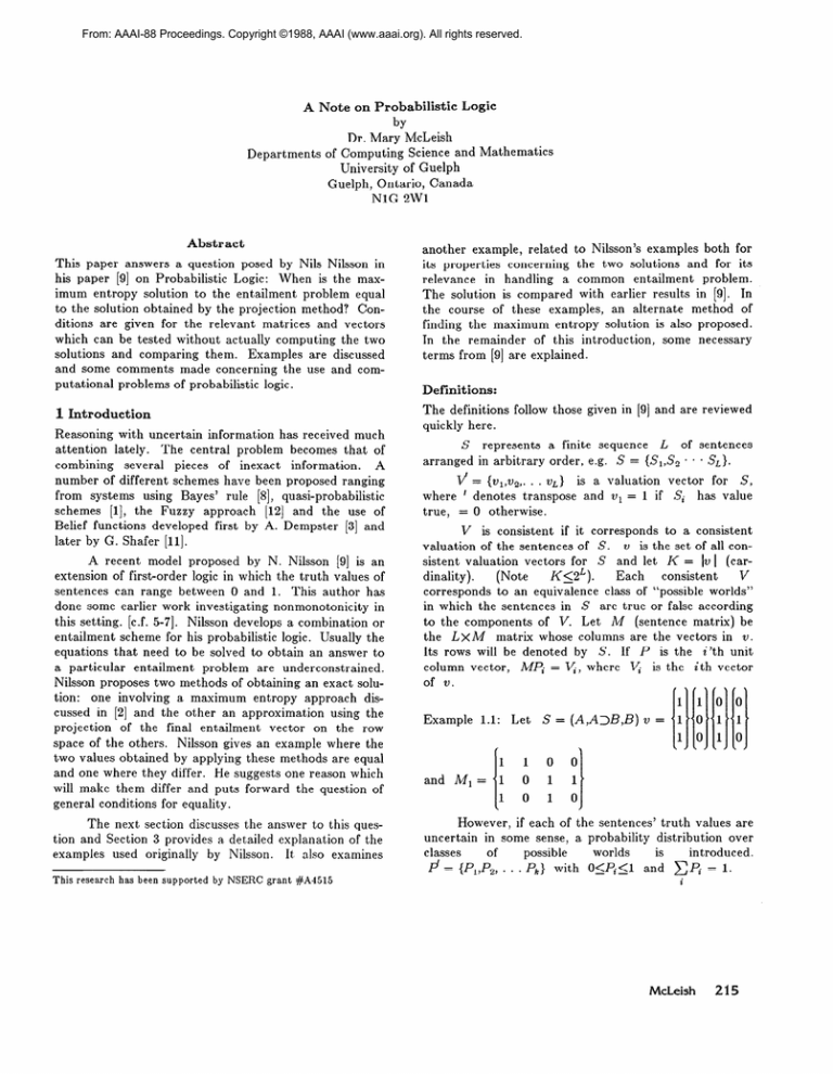
Example
1.1:
Let
S = (A,A>B,B)
v =
I11
0
1
1
0
1
0
1
0
1
1
0
1
0
However, if each of the sentences’ truth values are
uncertain in some sense, a probability distribution over
worlds
*
introduced.
possible
. . Pk} with O<Pi<l
ai:
c Pi = 1.
by NSERC grant #A1515
McLeish
215
Here the i’th component of P represents the probability that ‘our’ world is a member of the i ‘th class of
worlds. Now a consistent probabilistic valuation vector
V over the sentences in S is computed from the equation V = MP. The components of V are the probabilities of the Si being true (or the probability that ‘our’
world is a member of one of those classes of possible
worlds in which sentence Si is true).
Returning to example 1, we find that even if consistent valuations are known for the sentences A and
AIB, the probability of B is not necessarily uniquely
determine
the
bounds
defined.
One
can
p(A3B) + p(A)-l<p(B)<p(A1)I3),
which
provide
some restrictions. However, often a more precise value
for p(B) needs to be predicted. One method for doing
this is explained below.
Probabilistic
Entailment:
A method using a maximum entropy approach (borrowed from P. Cheeseman
[5]) is used to obtain an exact solution for p(B).
The entropy function becomes H = -P.log P + I,
(vI-S,.P)
+ Z2(v,-S2.P) + . * * ZL(vL-SL.P), where the
Zi are Lagrange multipliers. Following Cheeseman, the
solution for maximum entropy becomes
pi = e-‘*e-wd
......e-wLil
If one employs this method, at least for example 1, the
solution for
(N4/2)
9 = {P+P--l, l-q, (bw4
,
when v’ = (1, p, q} and thus p(B) = p/2 + q-l/“.
Projection
Method:
Another method uses an approximation of B by S”, the projection of B onto the row
space of Ivr’= M, with the last row deleted and a row
of l’s inserted at the top. Then S* = cc;S;
and
S* . P = CCi~.
Applied
to the example
given,
S* = (l,O,?h , %)
and
P(S”) = f
+ q - $ = p(B)
using the max entropy solution.
However, the entailment example of A,B,Ar) B is
given in [9] and here the two methods give different solutions. The following section addresses the problem of
why this happens.
2 Conditions
for Equality
of the Two
Solutions
From the example used in PI of the entailment of A,B
and An B, it is seen that P
) from max entropy
= pq (where p(A) = p , p(B) =‘qj and from the projec1
tion method the result is ;+;-7.
Nilsson rightly
(47B
states that these two quantities cannot be equal when
the max entropy solution contains a product because the
solution obtained from the projection method will always
be a linear combination of the 6 (here, l,p,q).
Thus,
216
Automated Reasoning
knowledge of the maximum entropy solution is sufficient
to answer the equality question. Let us state this formally as a first condition. Let P stand for the solution
vector for M’X = V obtained using maximum entropy.
2.1:
Only if the maximum entropy solution P
can be written as a linear combination of the vectors Vi
can S*P = cc;Vi,
where S” = ~c;S~ is the projection
Theorem
of S on the row space of d.
To explain the reasons for this more fully and find conditions not requiring the computation of P, let us look at
some matrix algebra theory.
If the row vectors of A/ are not linearly independent, they can be reduced to an independent set by
Consider
then
ones.
unessential
dropping
any
This matrix has the pro erties of a generalM(tiM)-‘.
ized inverse of hl’ (referred to as (h B)-. [c.f. lo]. Now if
P = M(dM)-‘V,
it will solve A/X = V. (This mea.ns
P is a linear combination of the v). As S**Q = CC;~
for any solution Q to &X = V, then S**M(hiAd)-‘V
must be the solution from the projection method to the
S.P = SM(M%)-‘V
Now
problem.
entailment
= S*M(~M)-‘&IP
= S*P (S and S* are now row vectors). This shows that if P is a particular linear combination of the vi, the solutions are the same. Some other
obvious results hold and will be stated before more general results are given.
Lemma
cal.
2.2:
If P = (ha)-V, the 2 solutions are identi-
2.3: If S”*P = S-P the 2 solutions are identical.
This follows from a remark above with P = (2.
Lemma
Lemma
2.4:
If S = S” the 2 solutions are identical.
If P = P* (the projection of the max
2.5:
entropy vector on the row space of A/), the two solutions are equal.
This f .50110ws from S*P = S*M(lfM)-‘&iP
= s*p.
Lemma
What is the general solution to A/X = V? From
[4,10], it can be seen to be a particular solution plus any
linear combination of solutions to the homogeneous equation. One way to express this is as (h/l)- +(H-I)Z,
where 2 is arbitrary and H = (d)-&.
Solutions may
also be obtained to the homogeneous equation by first
row reducing M’ to a form in which the first T column
vectors are independent.
Then W, = (the P + l’st column, -l,O, * * . ,O)
W, = (the T + 2nd column, 0,-l, * * . ,0)
etc.
W n7 = (the 12th column, O,O, * . * ,-1).
Here
di~n(&)
= m x n and M’ is assumed to ha.ve rank
r.
must be related
Thus P and P1 = M(i’bfM)-‘V
Thus
according to P = PI + (wi , 20~ , * * * , zu,,).Z.
But
s P = S-P, + qw,
, 202, . * * ) w,,).Z.
S-P1 = S”*P1 (as the projection of P, on the row space
of M, equals itself). Therefore the 2 solutions are equal
if and only if S(wi , w2, * * * , w,,)
= 0 or S is
orthogonal to the space of homogeneous solutions unless of course P = P,, when the 2 solutions are clearly
equal (2 is then identically 0). From matrix theory this
implies S lies in the row space of fit. The above actually
proves the following result:
Theorem
2.6: The max entropy and projection solutions are equal if and only if either P = (&)-If
or
s* = s.
Clearly the second condition is easy to check, however the first requires the full computation of P. However, if we consider how the maximum entropy solution
is formed we can find an easier condition to check. Suppose & can be transformed by simple row operations
(not the full Gram-Schmidt process which involves vector products of the ro)vs) to the form (I C), where I is
an rxr unit matrix and C contains at most one 1 in any
column. The row vectors are the orthogonal.
M’ may
always be row reduced to Mi = (I C) (if its rank is Y),
but C may not have this special form.
In this situation then, the max entropy solution
may be written as M, [a, * * * a,]’ , where the ai are the
special exponential variables used in the max entropy
solution [2]. Now M, [ai * . * a,]’ may be made equal to
M,(MiM,)-‘V,
by letting (a, * * * a,) = V, (V, is V
transformed appropriately when A/ was converted to
(I C).) The solution for the ui is unique and this solution
gives AdP = V. Thus P = (Mi)-V, = (h/o-V.
If A/ cannot be row reduced to the form just
described, one obtains pi = al , i = i , . * . T and then
Pj = products of the ai and hence the pi, for j > T and
i 5 T. If P = M(dM)-‘V,
this is not possible as all the
members of P are linear combinations of the Vi. Thus
we have result 2.7:
Theorem
2.7: P = (1M)-)V if and only if ILI’is row
reducible to the form (I C), where each column in C
contains at most one 1. (So C’ = C transpose is in
echelon form).
The next section discusses some examples in the
light of these results. The final results 2.G and 2.7 make
the discovery of the equality of the 2 solutions easy to
verify. The property required of hl’ could be stated in
terms of the existence of a transformation matrix which
will turn A/ into this form, but the conditions as given
are just as easy to verify. There are standard methods
of row-reducing Ad to (I C) and then it is just a
question of checking whether or not C has the desired
properties.
3 Examples
3.1
Consider
the
example
of
used in [9].
the
Ml =
It can be shown
max
entropy
that
solution
14)
[P+q-17
h?,
(l-P)/%
Cl-P)/21’.
Indeed, this could also be discovered by the fact that M’
11 0 0 01
can be row reduced to the echelon form 10 1 0 01
lo 0 1 l]
where the column vectors never contain more than one
non-zero entry (row vectors are orthonormal). Actually
B # S* and B*(O 0 1 -I), where (0 0 1 -1) = w1 is not
zero. However, the row reduction immediately gives the
max entropy variables (ai , a2 , aa)
/ \
‘q+p-1
I
q+p---l
as (h/(M)-1
l-q
-1-q
=
2
\ 1-P
1-P
2
produces
Then Mb1 a24
= (PI P2P3PJ
entropy solution shown above.
the
max
3.2.
Consider
the
example
S, = A , S2 = B , S, = AnB
given in [9]. Let S = S:f
1 1 1 1
A,/ =
1 1 0 0 ,
I
1
which
has
a
row-echelon
form
column of & : /5’= (-1 , 1 , 1 , -1) (See page 6, [lo]).
The dimension of the solution space should be n-r
where h/( is an mxn
matrix of rank r. So all homogeneous solutions are of the form kp for some constant
B.
Thus the max entropy solution and the solution
using the generalized inverse l-d- introduced earlier
differ by k(-1 , 1 , 1 ,-1).
The vector S is (1 0 0 0),
which is not orthogonal to kp. Thus the solutions for
p(S) will not be the same. One could also check that S
McLeish
217
A (Tweety)
V x [Ax --) Bx]
B (Tweety)
is not in the subspace generated by the row vectors of
ti as N, th e matrix obtained by adding the row vector
S to the matrix M’ has non-zero determinant.
Note that this is not the same as the sequence:
3yA(y) , Vx[A(x) + B(x)] , (3z)(Bz)
represented
by
the M matrix in [9]. Nor is it the same as
It is interesting to see how the different solutions
are related.
/ \
The particular solution found by using the generalized inverse (A!@ is:
3
I I,
1
3
-1
-1
3
q--l+p
M(tiM)-’
l-q
1-P
=$
:
-1
1
1
/
S1 : A (Tweety)
S, : A (Tweety) --* B (Tweety)
S3 : B (Tweety) ,
cl--l-l-P
1 ,I
1-q
l---p
which was also investigated in [9] this. Let p , q and T
be the probabilities of S, , S2 and S3 respectively. So p
represents the probability Tweety is a bird (we are
assuming a universe of animals for example),
q
represents the probability
that all birds fly and T
represents the probability that Tweety flies.
1
\
2q + 2p - 1
1 -2q
=;i-
+ 2p + 1
2q-2p-F1
,-2q
=P1
.
Now M, the matrix of consistent vectors becomes,
-2p-G
1100100
Now P= ICI-1 1 1 -11’ + PI for some k.
= 4pq - i?, - 2p + ‘1 ’ *
k
, a solution is found.
4
Indeed
/
-1
a2
1
a3
=
k1
u2a3
\
1
1 1 0 0 1 0 0 , which can be reduced to
~~~e~~~~~~
i
i
fi
-1
:I.
ThereforePi
Consider
-1
Let
the
rows
of
#
be
b, , b2 , b3 , b,.
Then
-k + b, , a2 = k + b, , u3 = k + b3
and
then
(k + bJ(k + b3) = (-k + b,)(-k + bl), from which k
can be easily found and thus al , u2 and u3.
al=
For this M’ matrix then, the only way in which
S”*P1 = S*P is for S*(-1 1 1 -1)’ to be zero. This also
means that S should lie in the row space of M’ and equal
its own projection on this row space. If N is a square
matrix, then finding det(N) quickly produces an answer.
Otherwise, it is probably easier to compute the reduced
form of & and check if S*Wi = 0 for each of the Wi
computed from the last n-r
column vectors of the
i-1 00 *** 0)
reduced
form of hl’ by adding .
* * * -1) to thex’
’
3.3 As another example, consider the following scheme
where Ax : x is a bird, Bx : x flies, and consider the
entailment:
Automated Reasoning
1101
B*Wi, where
w1 = (0 0 1 -1 0 0 0) ,
0) ,
w3 = (-1
) 1 , 1 ) 0 0 -10) ,
w4 = (-1
1 10 0 0 -1) are the solutions to the homogeneous
equations.
(B = (1 0 1 0 1 1 0),
following
Nilsson’s
terminology
here).
Bw, = 0 , B.w2 = -1 , B*w3 = -1
and
B*w, = 0.
Therefore B-P will not equal B-P. Indeed, the projection of B on the row vectors of hr( is (.8 .6 .6 .6 .6 .4 .4),
(not a very good approximation).
The solution using the generalized inverse discussed ear-
w2 = (0 10 0 -10
+p1
a1
2i8
10
will not equal P.
L I
(0, -1 , 0 * * + 0). . . (0, 0,
1011000
110
This computation suggests that a max entropy
solution can always be found for k from the particular
and homogeneous solutions: (i.e.) using the reduced form
of &, the max entropy solution for the pi in terms of ai
(notation as in [9]), becomes
a1
I
if
lier is r’ =
2-l-p-l-q
The
5
.
very complicated resulting in
r=
max entropy
solution
is
(P+4)+~(P+c1)2+4(l--P)(1--cl)
4
When p = q = 1, T = I, unlike the solution T’, which
equals
.8,
not
a very
sensible
result.
When
1
a.nd r = T. These values represent
P =q=o,rLf
the probability
tweety flies if yt, is not a bird and not all
q = l,r’ = -3+P
and T = -$
+ PI*
5
The fact that T is greater than p is reasonable as this
mode1 allows for a non-zero chance that non-birds fly. It
is bounded below by % because if p = 0 (Tweety is not a
birds fly.
When
bird), T = %.
Note that the maximum entropy solution here does
have some properties which are more desirable than
using the system
S1 : A (Tweety)
S2 : A (Tweety) --* B (Tweety)
S3 : B (Tweety)
1
and the scheme in [S] giving r = E2 + (I - y.
P =q=o,r
p=o,r=q--$,
is
undefined
and
which could be negative.
PI
McLeish, M., “Nilsson’s probabilistic entailment
extended to Dempster-Shafer Theory”, Proc. of the
Uncertainty Management Workshop, Seattle, 1987,
(submitted to Uncertainty in A.I. Book, North Holland)
PI
McLeish, M. “Probabilistic logic: some comments
and possible use for nonmonotonic reasoning”, to
appear in Uncertainty in Arti jicial Intelligence
edited by J. Lemmer, North Holland, April, 1988.
PI
Duda, R.O., Hart, P.E., Nilsson, N.J., “Subjective
Bayesian methods for rule-based inference systems”, Proc 1976 National Computer Conference,
AFIPS, vol. 45, pp. 1075-1082.
PI
Nilsson, N., “Probabilistic Logic”, SRI technical
report #321 (1984) and Artificial Intelligence, vol.
28, Feb. (1986), pp. 71-87.
WI
Rao, C.R., “Linear Statistical Inference
Applications”, John Wiley, 1973.
111
Shafer, G.A., Mathematical Theory of Evidence,
Princeton University Press, Princeton, N. J. (1979).
P
Zadeh, L.A., “Fuzzy logic and approximate reasoning”, Synthese 30: (1975), pp. 407-428.
When
when
Of course,
which solution is the more acceptable depends on the
chosen interpretation in probabilistic logic of the problem being considered. If you have an animal and know
the probability of its being a bird, and know the probability that all birds fly and wish to discover if that
animal flies, then the scheme given here in example 3.3 is
reasonable.
4 Conclusions
This note has given the conditions under which the
maximum entropy and projection methods discussed in
[9] produce the some entailment results. These conditions can be applied without actually computing the two
solutions and comparing them.
and Its
It might be interesting to obtain an idea from the
general solution to the type of underconstrained equations encounted here to study p(S). That is, the possible
solutions for p(S) are S*(ILI(tiM)-‘V
+ (H - I)2 for
any vector 2 and this bracketed value may be computed
with relative ease. The maximum entropy solution will
be included amongst these values.
References.
PI
Buchanan, B.G., Shortliffe, E.H., Rule-based expert
systems, Addison-Wesley, (May, 1985).
PI
Cheeseman, P., “A method of computing generalized Bayesian probability values for expert systems”. Proc. Eighth International joint conference
on Artificial Intelligence, Karlsruhe, (1983) pp.
198-292.
PI
Dempster, A.P., “A generalization of Bayesian
inference”, Journal of the Royal Statistical Society,
series B, vol. 30, (19GS), pp. 205-247.
WI
Hoffmann,
I<., Kunze,
Prentice-Hall, 1970.
151
McLeish, M., “Dealing with uncertainty in nonmonotonic reasoning”. Proceedings of the Conference on Intelligent Systems with Machines, April
(1986), Oakland U., Michigan pp. l-5.
R.,
“Linear
Algebra”,
McLeish
219