Joint Recognition of Multiple Concurrent Activities
using Factorial Conditional Random Fields
Tsu-yu Wu and Chia-chun Lian and Jane Yung-jen Hsu
Department of Computer Science and Information Engineering
National Taiwan University
yjhsu@csie.ntu.edu.tw
Abstract
the home for varying lengths of time. Sensor data are collected as the occupants interact with digital information in
this naturalistic living environment. As a result, the House n
data set (Intille et al. 2006a) is potentially a good benchmark
for research on activity recognition. In this paper, we use the
data set as the material to design our experiment.
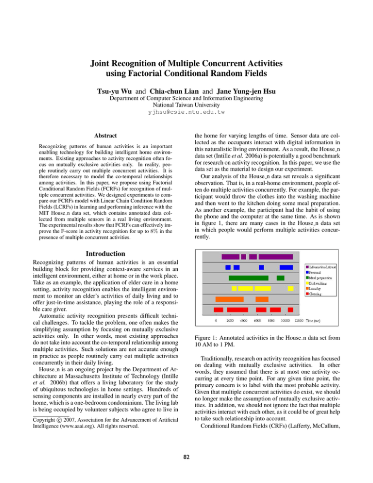
Our analysis of the House n data set reveals a significant
observation. That is, in a real-home environment, people often do multiple activities concurrently. For example, the participant would throw the clothes into the washing machine
and then went to the kitchen doing some meal preparation.
As another example, the participant had the habit of using
the phone and the computer at the same time. As is shown
in figure 1, there are many cases in the House n data set
in which people would perform multiple activities concurrently.
Recognizing patterns of human activities is an important
enabling technology for building intelligent home environments. Existing approaches to activity recognition often focus on mutually exclusive activities only. In reality, people routinely carry out multiple concurrent activities. It is
therefore necessary to model the co-temporal relationships
among activities. In this paper, we propose using Factorial
Conditional Random Fields (FCRFs) for recognition of multiple concurrent activities. We designed experiments to compare our FCRFs model with Linear Chain Condition Random
Fields (LCRFs) in learning and performing inference with the
MIT House n data set, which contains annotated data collected from multiple sensors in a real living environment.
The experimental results show that FCRFs can effectively improve the F-score in activity recognition for up to 8% in the
presence of multiple concurrent activities.
Introduction
Recognizing patterns of human activities is an essential
building block for providing context-aware services in an
intelligent environment, either at home or in the work place.
Take as an example, the application of elder care in a home
setting, activity recognition enables the intelligent environment to monitor an elder’s activities of daily living and to
offer just-in-time assistance, playing the role of a responsible care giver.
Automatic activity recognition presents difficult technical challenges. To tackle the problem, one often makes the
simplifying assumption by focusing on mutually exclusive
activities only. In other words, most existing approaches
do not take into account the co-temporal relationship among
multiple activities. Such solutions are not accurate enough
in practice as people routinely carry out multiple activities
concurrently in their daily living.
House n is an ongoing project by the Department of Architecture at Massachusetts Institute of Technology (Intille
et al. 2006b) that offers a living laboratory for the study
of ubiquitous technologies in home settings. Hundreds of
sensing components are installed in nearly every part of the
home, which is a one-bedroom condominium. The living lab
is being occupied by volunteer subjects who agree to live in
Figure 1: Annotated activities in the House n data set from
10 AM to 1 PM.
Traditionally, research on activity recognition has focused
on dealing with mutually exclusive activities. In other
words, they assumed that there is at most one activity occurring at every time point. For any given time point, the
primary concern is to label with the most probable activity.
Given that multiple concurrent activities do exist, we should
no longer make the assumption of mutually exclusive activities. In addition, we should not ignore the fact that multiple
activities interact with each other, as it could be of great help
to take such relationship into account.
Conditional Random Fields (CRFs) (Lafferty, McCallum,
c 2007, Association for the Advancement of Artificial
Copyright Intelligence (www.aaai.org). All rights reserved.
82
& Pereira 2001) provide a powerful probabilistic framework for labelling and segmenting structured data. By
defining a conditional probability distribution over label sequences given a particular observation sequence, CRFs relax
the Markov independence assumption required by Hidden
Markov Models (HMMs). The CRF model has been applied to learning patterns of human behavior (Chieu, Lee, &
Kaelbling 2006; Sminchisescu, Kanaujia, & Metaxas 2006;
Liao, Fox, & Kautz 2007). Nevertheless, as mentioned
above, previous research ignored the possible interactions
between multiple concurrent activities.
To address this problem, we advocate using a factorial
conditional random fields (FCRFs) (Sutton & McCallum
2004) model to conduct inference and learning from patterns
of multiple activities . Compared with basic CRFs, FCRFs
utilize a structure of distributed states to avoid the exponential complexity problem. In addition, the FCRF model accommodates the relationship among multiple concurrent activities and can effectively label their states.
This paper is organized as follows. At first, we introduce the CRFs and FCRFs model. And then we present
FCRFs for multiple concurrent activities recognition including the model design, the inference algorithm, and the learning method. Finally, we describe our experiment for performance evaluation of this model, followed by the conclusion
and future work.
Figure 2: An LCRF example for activity recognition.
Figure 2 shows an example of applying linear chain CRFs
(LCRFs) to activity recognition. We can represent the states
of activities as a time sequence. Thus, we have a set
of hidden variable nodes Y = {Y 1 , Y 2 , Y 3 . . .} standing
for the activity sequence. Given the observation sequence
X, the dependency can be defined by the feature functions upon the cliques. Several researchers have applied
CRFs to activity recognition (Chieu, Lee, & Kaelbling 2006;
Sminchisescu, Kanaujia, & Metaxas 2006; Liao, Fox, &
Kautz 2007) , but they did not address the issue of multiple concurrent activities.
To recognize multiple concurrent activities, it is possible to construct a unique model for each individual activity.
However, this approach ignores the relationship between different activities. For example, the House n data set (Intille
et al. 2006b) shows that the participant often used the phone
and the computer concurrently in the experiment. In addition, a person typically cannot sleep and watch TV at the
same time.
To take the co-temporal relationship between multiple activities into account, we may treat each combination of multiple activities as a new activity. However, the model complexity of this approach grows exponentially with the number of activities to be recognized. As a result, inference and
learning may become computationally intractable when the
number of activities is large.
Factorial CRFs (FCRFs) (Sutton & McCallum 2004),
which are like Factorial HMMs (FHMMs) (Ghahramani &
Jordan 1997), suggest a structure of distributed states to
avoid the exponential complexity problem. In addition,
FCRFs can model the dependency between multiple concurrent activities by introducing co-temporal connections.
Conditional Random Fields
CRFs are undirected graphical models conditioned on observation sequences which have been successfully applied
to sequence labelling problems such as bioinfomatics (Sato
& Y. 2005; Liu et al. 2005), natural language processing
(Lafferty, McCallum, & Pereira 2001; Sha & Pereira 2003;
Sutton & McCallum 2004; Sarawagi & Cohen 2005) and
computer vision (Sminchisescu, Kanaujia, & Metaxas 2006;
Vishwanathan et al. 2006).
Unlike generative models such as Dynamic Bayesian Networks (DBNs) and HMMs, CRFs are conditional models
that relax the independence assumption of observations and
avoid enumerating all possible observation sequences. Maximum Entropy Markov Models (MEMMs) are an alternative
conditional models, but they suffer from the label bias problem (Lafferty, McCallum, & Pereira 2001) due to per-state
normalization. In contrast, CRFs are undirected structures
and globally normalized, thereby solving the label bias problem.
Let G be an undirected graph consisting of two vertex
sets X and Y , where X represents the set of observed random variables and Y represents the set of hidden random
variables conditioned on X. Given graph G, let C be the set
of maximum cliques, where each clique includes vertices
Xc ∈ X and Yc ∈ Y . For a given observation sequence
Y , CRFs define the conditional probability by the potential
function Φ(Xc , Yc ) such that
1 Y
P (Y |X) =
Φ(Xc , Yc )
Z(X)
An FCRFs Model for Multiple Concurrent
Activities Recognition
Model Design
Let Yit be a random variable whose value represents the
state of activity i at time t and Y t = {Y1t , Y2t . . . YNt }
where N is the number of activities to be recognized. In
a total time interval T , let Y = {Y 1 , Y 2 . . . Y T } be a sequence of vector Y t . We can define the observation sequence X = {X 1 , X 2 . . . X T } in the same way. Suppose
that there is a graph G = {V, E}. Let each element in Y t
c∈C
where Z(X) is the normalization constant.
83
and X t be a vertex in G. Edges in G represent the relationships between these random variables.
Figure 3 shows a sample FCRF model for recognition of
three concurrent activities. The FCRF is represented in a
dynamic form by unrolling the structure of two time slices.
There are two sets of edges standing for different relational
meanings. The edge set Ec , which includes pairs of activity
variables in the same time slice, represents the co-temporal
relationship; the edge set Et , which includes pairs of activity variables across time slices, represents the temporal
relationship.
Inference Algorithm
Given any observation sequence O, there are two kinds of
inference tasks of concern. One task is to compute the
marginal probability of each node pair, which will be used in
the learning algorithm to be introduced later. The other task
is to perform MAP (Maximum A Priori) inference to infer
the most possible sequence of activities states.
There are many inference algorithms for CRFs, including the forward-backward algorithm, mean field free energy, junction tree, and loopy belief propagation (LBP),
which is one of the most popular CRFs inference methods.
Even though it can only approximate the probabilities and
does not guarantee convergence for graphs with loops, LBP
has been shown to be effective (Sutton & McCallum 2004;
Vishwanathan et al. 2006; Liao, Fox, & Kautz 2007).
Sum-Product Algorithm To compute the marginal probability, the LBP sum-product algorithm is adopted. We introduce a “message” mij (Aj ) for each pair of neighboring
nodes Ai and Aj , which is a distribution sent from node
Ai to node Aj about which state variable Aj should be in.
All messages mij (Aj ) are initialized as uniform distributions over Aj . The message mij (Aj ) sent from node Ai to
its neighbor Aj is updated based on all the messages to Ai
received from its neighbors An except those from node Aj .


X
Y
Ψ(Ai , O)Φ(Ai , Aj , O)
mij (Aj ) = κ
mki (Ai )
i
Figure 3: An FCRF example of three concurrent activities.
where Ψ(Ai , O) is the local potential, Φ(Ai , Aj , O) is the
pair-wise potential, and κ is the normalization constant.
The messages propagate through the CRF graph until
they converge, when every message varies for less than a
threshold. Given that LBP does not guarantee convergence,
we have to set a limit on the maximum number of iterations. Even though the update order of messages may affect
the convergent speed, empirical study (Sutton & McCallum
2004) showed that a random schedule is sufficient.
After LBP converges, the marginal probability of nodes
Ai and Aj is then determined as
Y
Y
P (Ai , Aj ) = κ0 Θ(Ai , Aj , O)
mki (Ai )
mlj (Aj )
We define pair-wise potential functions Φc (Yit , Yjt , X)
for each edge (Yit , Yjt ) in Ec and Φt (Yit , Yit+1 , X) for each
edge (Yit , Yit+1 ) in Et . And we define the local potential
function Ψ(Yit , X) for each vertex Yit in G. The FCRFs will
be determined as


T N
1 Y Y
Φc (Yit , Yjt , X)
p(Y |X) =
Z(X) t=1 i,j
TY
−1 Y
N
t=1
!
Φt (Yit , Yit+1 , X)
T Y
N
Y
!
Ψt (Yit , X)
k6=i,j
t=1 i
i
where Z(X) is the normalization constant.
The potential functions Φc , Φt and Ψ are then defined
by a set of feature functions f = {f1 , f2 . . . fK } and their
corresponding weights λ = {λ1 , λ2 . . . λK } such that
!
X
t
t
t
t
Φc (Yi , Yj , X) = exp
λk fk (Yi , Yj , X)
Θ(Ai , Aj , O) = Ψ(Ai , O)Ψ(Aj , O)Φ(Ai , Aj , O)
k enumerates over all neighbors of Ai , l enumerates over all
neighbors of Aj and κ0 is the normalization constant.
MAP Inference To do MAP inference, we replace summation with maximization in the message update rule of the
sum-product algorithm. We have


Y
mij (Aj ) = κ max Ψ(Ai , O)Φ(Ai , Aj , O)
mki (Ai ) ,
!
X
λk fk (Yit , Yit+1 , X)
k
!
Ψ(Yit , X)
= exp
X
l6=i,j
where
k
Φt (Yit , Yit+1 , X) = exp
k6=i,j
λk fk (Yit , Yit , X)
i
k
where κ is the normalization constant.
Now, we have formally defined the FCRFs.
84
k6=i,j
After LBP converges, the MAP probability of node Ai is
defined as
Y
P (Ai ) = Ψ(Ai , O)
mji (Ai ),
for each parameter λk so that we maximize
the penalized
P
log-likelihood L(λ|D) = L(D|λ) + k logP (λk ). As a
result, the partial derivative becomes
∂L(D|λ) λk
∂L(λ|D)
=
− 2.
∂λk
∂λk
σ
j6=i
where Aj is the neighbor of Ai .
To do the inference, we can label every hidden variable by
choosing the most likely value according to the MAP probability.
Experiments
We have introduced the FCRFs model for multiple concurrent activities recognition. Let us find out how it works for
the House n data set. In this section, we describe the experimental design as well as the experimental result for the
evaluation of our model.
Learning Algorithm
The purpose of learning is to determine the weight λk for
each feature function fk . We can do this by maximizing the
log-likelihood of the training data. Given the training data
D = {A(1), O(1); A(2), O(2) . . . A(M ), O(M )}, the loglikelihood L(D|λ) is defined as follows.
X
L(D|λ) =
log P (A(m)|O(m))
Experimental Design
We extracted our experimental data from the MIT House n
data set, which is freely available for academic research.
The data set was recorded on Friday March 4, 2005 from
9 AM to 1 PM with a volunteer performing a set of common household activities. The data set recorded the information from a variety of digital sensors such as switch sensors, light sensors, and current sensors, etc. The data set was
then manually labelled with ground truths of multiple activities and location information. Unfortunately, with only four
hours of recorded activities in the released data set, the sensor data were too sparse to be useful for effective training.
As the House n data are still being collected, cleaned, and
labelled, so more comprehensive data set may be forthcoming. Meanwhile, we decide to utilize the location data as our
primary observations. The location information in the current House n data set is manually annotated and assumed to
be quite accurate. Nevertheless, our system should perform
in the same way should such data come from some (roomlevel) indoor location tracking system.
Now, let’s explain the data used in our experiments in
more detail. The annotation of the data recorded from 9 AM
to 10 AM is somewhat unorganized, so we decided to use
only the data set recorded from 10 AM to 1 PM for a total
of 10800-second. We labeled the activities for every second and divide the data set into 18 parts, each containing 10
minutes of data. This way, we can do 6-fold cross-validation
for the evaluation. For simplicity, we clustered the original
89 activities into 6 classes of activities, including cleaning,
laundry, dishwashing, meal preparation, personal and information/leisure. Because the 6 classes of activities may overlap with each other, the property of multitasking is suitable
for our multiple concurrent activities recognition. In addition, there are 9 mutually exclusive locations that may be
observed, including living room, dining area, kitchen, office,
bedroom, hallway, bathroom, powder room and outside.
Our FCRFs model is constructed in the following way.
First, for each activity class, we build one hidden variable node which contains a Boolean state representing either happening or not-happening. And then we let all the
hidden variable nodes in the same time slice to be fully connected, assuming that every activity has cotemporal relationship with each other. To represent the temporal relationship,
we connect the two hidden variable nodes across two time
slices for the same activity class. In addition, we connect
m
The partial derivative of the log-likelihood with respect to
λk is derived as
∂L(D|λ) X X
fk (A(m)i , A(m)j , O(m))
=
∂λk
m i,j
−
XX
m
p(A(m)i , A(m)j |λ)fk (A(m)i , A(m)j , O(m)),
i,j
where edge (Ai , Aj ) can be either in Ec or Et .
The former part of the partial derivative is easy to compute, while the latter part can be difficult. The marginal
probability for the latter part can be computed by using
loopy belief propagation introduced in the previous subsection. As solving the equation ∂L(D|λ)/∂λk = 0 does not
yield a closed-form solution, λ may be updated iteratively
using some optimization techniques such as iterative scaling, gradient descent, conjugate gradient or BFGS (Wallach
2003; Sha & Pereira 2003) to find the weights that maximize
the log-likelihood.
Previous research has shown that L-BFGS works well in
such an optimization problem for CRFs learning and many
current CRFs packages implement this method. L-BFGS is
a variant of the Newton’s method, which is a second order
optimization method. It is computationally expensive to calculate the second order derivative, Hessian matrix, Newton’s
method. BFGS provides an iterative way to approximate
Hessian matrix by updating the matrix in the previous step.
L-BFGS implicitly updates the Hessian matrix by memorizing the update progress and gradient information in the previous m steps. As a result, L-BFGS can reduce the amount
of memory and computation needs.
In practice, L-BFGS requests the partial derivative as well
as the log-likelihood at each iteration. So far, we have explained how to compute partial derivative. As to the loglikelihood, computing the normalization constant directly is
infeasible, so we use Bethe free energy (Yedidia, Freeman,
& Weiss 2003) to approximate the normalization constant.
In order to reduce over-fitting, we define a zero mean
Gaussian prior P (λk ) = exp(−λ2k /2σ 2 ) with variance σ 2
85
every hidden variable node with one observed variable node
which represents the states of location.
The FCRFs model defined are used to do learning and inference for multiple concurrent activities recognition in our
experiments. The variance of the Gaussian prior is 9. To
evaluate the importance of co-temporal relationship between
activities, we constructed 6 linear chain CRFs (LCRFs)
models as for comparison. Each LCRFs model recognizes
only one activity class at a time.
In addition, we may extend our activity model to represent
long-range temporal dependency as well as the relationship
among different activities across time slices. In our current
implementation, both learning and inference are performed
off-line. To deploy activity inference in real-world contextaware applications, we will need to develop online inference
such as the CRF-filter algorithm proposed in (Limketkai,
Liao, & Fox 2007).
References
Performance Evaluation
Chieu, H. L.; Lee, W. S.; and Kaelbling, L. P. 2006. Activity recognition from physiological data using conditional
random fields. Technical report, SMA Symposium.
Ghahramani, Z., and Jordan, M. I. 1997. Factorial hidden
markov models. Machine Learning 29(2-3):245–273.
Intille, S. S.; Larson, K.; Tapia, E. M.; Beaudin, J. S.;
Kaushik, P.; Nawyn, J.; and Rockinson, R. 2006a. House n
placelab data set ( http://architecture.mit.edu/house n/data
/placelab/placelab.htm ).
Intille, S. S.; Larson, K.; Tapia, E. M.; Beaudin, J. S.;
Kaushik, P.; Nawyn, J.; and Rockinson, R. 2006b. Using a live-in laboratory for ubiquitous computing research.
In Fishkin, K. P.; Schiele, B.; Nixon, P.; and Quigley, A.,
eds., PERVASIVE 2006, volume l, 349–365.
Lafferty, J.; McCallum, A.; and Pereira, F. 2001. Conditional random fields: Probabilistic models. for segmenting and labeling sequence data. In Proceedings of the
Eighteenth International Confernence on Machine Learning (ICML-01).
Liao, L.; Fox, D.; and Kautz, H. 2007. Extracting places
and activities from gps traces using hierarchical conditional
random fields. International Journal of Robotics Research
26:119–134.
Limketkai, B.; Liao, L.; and Fox, D. 2007. Crf-filters: Discriminative particle filters for sequential state estimation.
In 2007 IEEE International Conference on Robotics and
Automation.
Liu, Y.; Carbonell, J. G.; P., W.; and V., G. 2005. Segmentation conditional random fields (scrfs): A new approach
for protein fold recognition. In Research in Computational
Molecular Biology, 9th Annual International Conference.
Sarawagi, S., and Cohen, W. W. 2005. Semi-markov conditional random fields for information extraction. In Advances in Neural Information Processing Systems 17.
Sato, K., and Y., S. 2005. Rna secondary structural alignment with conditional random fields. In ECCB/JBI (Supplement of Bioinformatics).
Sha, F., and Pereira, F. 2003. Shallow parsing with conditional random fields. In Proceedings of the 2003 Human Language Technology Conference and North American Chapter of the Association for Computational Linguistics.
Sminchisescu, C.; Kanaujia, A.; and Metaxas, D. 2006.
Conditional models for contextual human motion recognition. Comput. Vis. Image Underst. 104(2):210–220.
We want to test if the LCRFs model and the FCRFs model
can correctly predict the activity sequences in the testing
data set. There are 6 activities labels at each time stamp.
The value of each activity label can be either positive (for
happening) or negative (for not-happening. In each part of
the testing data set, there are 600 seconds and total 3600 activities labels. A label is considered to be True Positive (TP)
if the model correctly predicts its value to be positive. Similarly, a model is True Negative (TN) if the model correctly
predicts the value as negative. On the contrary, the label is
considered to be False Positive (FP) if the model wrongly
guesses the value as positive and False Negative (FN) if the
model wrongly guesses the value as negative. To evaluate
our performance, we calculate the recall, precision and Fscore for these two models.
The results are summarized in Table 1, which compares
the recall, precision and F-score for the testing data set.
Data set
FCRF(%)
LCRF(%)
Recall
48.2
34.3
Precision
51.5
53.3
F-score
49.8
41.7
Table 1: Performance Comparison of LCRFs and FCRFs.
As we can see, the FCRFs model outperforms the LCRFs
models. Even though the location information may be ambiguous for the recognition of activity, the consideration for
co-temporal relationship in FCRFs complements this deficiency. As a result, the proposed FCRFs model improves
the F-score up to 8%. This experimental result provides us
the conclusion that it is helpful to utilize the co-temporal relationship for activity recognition.
Conclusion and Future Work
This paper proposes the FCRFs model for joint recognition
of multiple concurrent activities. We designed the experiments based on the MIT House n data set and compared our
FCRFs model with the LCRFs model. The initial experiment showed that FCRFs improve the F-score for up to 8%
for recognition of multiple concurrent activities in daily living.
The current experiment presents just an initial step towards concurrent activity recognition. As we mentioned earlier, using a single sensor such as location may not be sufficient for disambiguating among the activities. To further
improve the recognition accuracy, data from multiple heterogeneous sensors must be combined and taken into consideration in any practical activity recognition system.
86
Sutton, C. A. Rohanimanesh, K., and McCallum, A. 2004.
Dynamic conditional random fields: factorized probabilistic models for labeling and segmenting sequence data. In
Proceedings of the Twenty First International Confernence
on Machine Learning (ICML-04).
Vishwanathan, S. V. N.; Schraudolph, N. N.; Schmidt,
M. W.; and Murphy, K. 2006. Accelerated training of
conditional random. fields with stochastic meta-descent.
In Proceedings of the Twenty Third International Confernence on Machine Learning (ICML-06).
Wallach, H. M. 2003. Efficient training of conditional
random fields. In Proceedings of the 6th Annual CLUK
Research Colloquium. University of Edinburgh.
Yedidia, J. S.; Freeman, W. T.; and Weiss, Y. 2003. Understanding Belief Propagation and its Generalizations. Kaufmann, M. chapter 8, 236–239.
87