Learning Models from Temporal-Logic Properties via Explanations
Miguel Carrillo and David A. Rosenblueth
Instituto de Investigaciones en Matemáticas Aplicadas y en Sistemas
Universidad Nacional Autónoma de México
Apdo. 20-726, 01000 México D.F.
Mexico
Abstract
that demonstrates why the formula representing such a property does not hold in the model. Hence, to make the formula
hold true, we must modify at least the part of the model generating such a path. Once modified, we can ask the model
checker again if the new model satisfies the property.
We are interested in mechanizing this transformation process of the given model. Of the many temporal logics used
in model checking, we selected “computation-tree logic”
(CTL) (Clarke, Grumberg, & Peled 1999), because of its
simple model-checking algorithm compared with that of
other logics. Moreover, motivated by some practical applications (Espinosa-Soto, Padilla-Longoria, & Alvarez-Buylla
2004), we limit ourselves to models having the same set of
states as that of the faulty, given model.
Given a model and a property expressed in temporal logic, a
model checker normally produces a counterexample in case
the model does not satisfy the property. This counterexample is meant to serve as a guide for manually modifying the
model so that the new model does satisfy the property. We
observe that basing the modification of a model on negative
information (why a formula is not true) can have limitations,
and we present a method employing positive information instead. Our method incrementally learns a subformula and
marks the part of the model that makes the already learned
subformula true (i.e. an explanation). Next, our method attempts to learn the rest of the formula without altering the
marked part of the model.
Introduction
Computation-Tree Logic
Model checking (Clarke, Grumberg, & Peled 1999) is a collection of techniques for verifying properties of systems having an ongoing interaction with the environment. A model
checker has as input a model representing a system and a
temporal-logic formula expressing a desirable property. The
output is either a confirmation or a denial that the property
holds. In case of denial, the model checker normally produces a counterexample, consisting of a part of the model
that makes the formula false. This counterexample is intended as a guide for manually modifying the model so that
the violated property is satisfied. Our objective will be to
study a method for automatically modifying a faulty model
using explanations instead of counterexamples.
Industry has increasingly been using model-checking
methods for at least two reasons. First, model checking can often detect faults eluding more traditional methods such as testing. Second, state-of-the-art implementations of model checkers, employing binary decision diagrams (Bryant 1992), allow the verification of properties in
systems with many states. Model checking has thus found
numerous applications, such as verifying digital circuits, developing critical software, and more recently exploring biological systems.
One of the most appreciated features of model checkers is
their ability to generate a counterexample if the model does
not satisfy a given property. Such a counterexample is a path
Definition 1. Given a finite set Prop of propositional variables, a Kripke structure or model M = S, R, L consists of a finite set S of states, a total relation R ⊆ S 2
over S (i.e. for every s ∈ S there exists t ∈ S such that
(s, t) ∈ R), called the accessibility relation, and a labelling
function L : S → 2Prop .
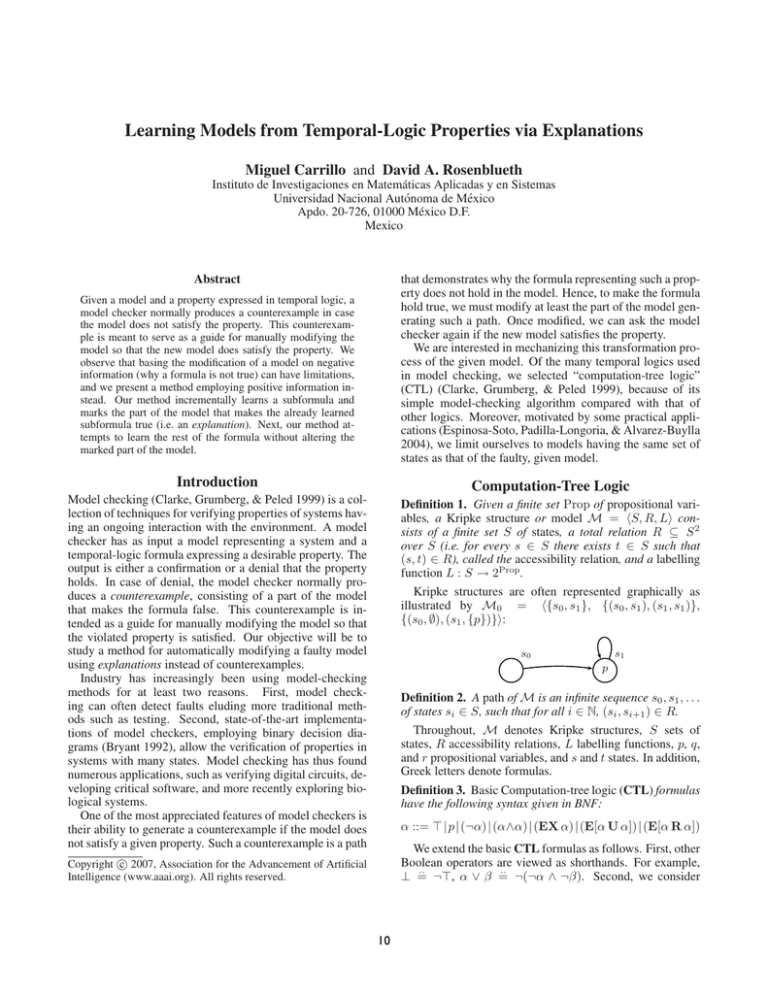
Kripke structures are often represented graphically as
illustrated by M0 = {s0 , s1 }, {(s0 , s1 ), (s1 , s1 )},
{(s0 , ∅), (s1 , {p})}:
s0
p
s1
Definition 2. A path of M is an infinite sequence s0 , s1 , . . .
of states si ∈ S, such that for all i ∈ N, (si , si+1 ) ∈ R.
Throughout, M denotes Kripke structures, S sets of
states, R accessibility relations, L labelling functions, p, q,
and r propositional variables, and s and t states. In addition,
Greek letters denote formulas.
Definition 3. Basic Computation-tree logic (CTL) formulas
have the following syntax given in BNF:
α ::= |p | (¬α) | (α∧α) | (EX α) | (E[α U α])| (E[α R α])
We extend the basic CTL formulas as follows. First, other
Boolean operators are viewed as shorthands. For example,
..
..
⊥ = ¬, α ∨ β = ¬(¬α ∧ ¬β). Second, we consider
c 2007, Association for the Advancement of Artificial
Copyright Intelligence (www.aaai.org). All rights reserved.
10
NNF can be readily obtained by repetitively pushing the
negation symbol to the atomic level and replacing each operator by its dual. For instance ¬EX p is converted to AX ¬p.
It is easy to see that this process obtains an NNF formula
equivalent to a given CTL formula.
A model-checking or model-synthesis algorithm would
have as input a formula in NNF. Hence, such an algorithm
must treat the dual operators as primitive operators.
The following equivalences (Clarke, Grumberg, & Peled
1999, p 63), (Huth & Ryan 2004, p 217) are instrumental for
such a model-checking or model-synthesis algorithm:
a number of dual temporal operators, whose definition can
be obtained by negating the operands and simultaneously
replacing A by ¬E, U by R, and R by U.
Definition 4. Extended CTL formulas are the basic CTL
formulas together with (1) ordinary Boolean operators, (2)
..
..
the following duals: AX α = ¬EX ¬α, A[α U β] =
..
¬ E[¬α R ¬β], and A[α R β] = ¬ E[¬α U ¬β], and
..
(3) the following particularizations: EF α = E[ U α],
..
..
..
EG α = E[⊥ R α], AF α = A[ U α], and AG α =
A[⊥ R α].
Mnemotechnically, the letters E and A denote Exists and
for All, respectively. The letters X, U, and R, in turn, abbreviate “neXt state,” “Until,” and “Release,” respectively.
E[α U β]
E[α R β]
A[α U β]
A[α R β]
Definition 5. (Semantics)
•
•
•
•
•
M |=s .
M |=s p iff p ∈ L(s).
M |=s ¬α iff M |=s α.
M |=s α ∧ β iff M |=s α and M |=s β.
M |=s EX α iff there exists a path s0 , s1 , . . ., where s0
equals s, such that M |=s1 α.
• M |=s E[α U β] iff there exists a path s0 , s1 , . . ., where
s0 equals s, and a j ≥ 0 such that for all i < j, we have
M |=si α and M |=sj β.
• M |=s E[α R β] iff there exists a path s0 , s1 , . . ., where
s0 equals s, such that either there is some i ≥ 0 such that
M |=si α and for all 0 ≤ j ≤ i we have M |=sj β, or
for all k ≥ 0, we have M |=sk β.
≡
≡
≡
≡
β ∨ (α ∧ EX E[α U β])
β ∧ (α ∨ EX E[α R β])
β ∨ (α ∧ AX A[α U β])
β ∧ (α ∨ AX A[α R β])
(1)
(2)
(3)
(4)
These apparently circular definitions can be used to define
the four operators on the left in terms of EX and AX by
means of fixed points of predicate transformers. The resulting algorithm computes all the states of the model in which
a formula holds.
Alternatively, we could also compute one state at a
time, and use a cycle-detection mechanism, instead of fixed
points. Our model-synthesis method will parallel such a
model-checking algorithm.
Explanations
In CTL model checking, counterexamples are generated
only for “universal” CTL formulas, i.e. those with operators starting with an A. Consider for example AF α, which
holds in state s iff for all paths starting in s there is some
state in which α holds. If AF α does not hold in state s,
then there is a path starting in s such that α is false in all
states of such a path. This path will be a counterexample.
Consider by contrast EF α, which holds in state s iff there
is a path starting in s having a state in which α holds. If
EF α does not hold in state s, then there is no path starting in s having a state in which α is true. Therefore, all
paths starting in s will be counterexamples. Instead of generating any one such path, the NuSMV model checker, for
instance, gives more information by returning s only. In case
of formulas with nested universal and existential operators,
NuSMV produces a path prefix ending in a state in which
the outermost existential formula does not hold. As a result, universal operators occurring inside an existential operator provide no information to the counterexample. This
drawback of counterexamples suggests considering “explanations” instead.
Following the CTL model-checking algorithms of (Huth
& Ryan 2004), we can learn first the smallest subformulas
and work towards the main formula. Explanations allow us
to learn conjunctions α ∧ β of formulas as follows. We first
inductively learn α. Next, we find an explanation for α and
“protect” such an explanation. Finally, we learn β in such
a way that the explanation for α is preserved. (Learning β
might involve the addition or removal of transitions or labels.) We will then have learned both conjuncts.
In the model M0 above, for example, M0 |=s0 EX p and
M0 |=s0 EF p hold, but M0 |=s0 p does not. In addition,
M0 |=s1 EG p and M0 |=s0 EX AG p hold, but M0 |=s0
AG p does not.
Negation Normal Form
Given a Kripke structure M = S, R, L, a CTL formula
α, and a state s, we are interested in modifying R and L,
obtaining M = S, R , L , in such a way that M |=s α
holds, if possible. Compared with the model-checking problem (determining whether or not M |=s α holds) we have
an important variation. Sometimes model checkers for CTL
solve the more general problem of computing all states s of
the model M satisfying α (Huth & Ryan 2004, p 222). This
allows the possibility of viewing negation as the set difference w.r.t. the set of states of the model.
In our case, computing the set of all models M with the
same set S of states, such that M |=s α holds, would also
allow us to view negation as set difference, but would be intolerably inefficient, as there is a vast number of such models. Consequently, we will not treat arbitrary occurrences of
negation. By contrast, if we limit ourselves to negation applied to atomic formulas, it is possible to treat negation directly, as we will see. This implies, however, having to transform arbitrary CTL formulas to “Negation Normal Form.”
Definition 6. An extended CTL formula is in Negation Normal Form (NNF) iff “¬” is applied only to atomic formulas.
11
Finally, we deal with and ⊥. The explanation for ,
the identity for conjunction, is the identity for the union of
explanations, i.e. the empty explanation ∅, ∅, ∅. The explanation for ⊥, the identity for disjunction, is the identity for
nondeterministic choice, i.e. the undefined explanation E⊥ .
An algorithm for computing explanations
Let us consider a possible definition of explanations. Given
a model M = S, R, L in which a formula α holds, an
explanation for α would be a minimal part of the model that
makes α true.
Take for instance the model M0 above. An explanation
for the truth of p at the state s1 of M0 given that M0 |=s1 p
holds, would be the label p in state s1 . Hence, for representing explanations for atomic formulas (i.e. positive literals),
we need L ⊆ S × Prop.
In the case of a negative literal, consider M0 |=s0 ¬p. If
we record the occurrence of negative literals in states (i.e.
(s0 , ¬p)), we will have a symmetrical situation to that of
positive literals, and we will be able to handle negation (of
atomic formulas). Hence, in addition to recording positive,
we will record negative literals: L ⊆ S × Lit, where Lit is
the set of literals of Prop.
In the case of a conjunction α ∧ β, we would need to explain first α, then β, and finally obtain the “union” of both
explanations. As we have not yet finished describing the
components of an explanation, we will relegate the definition of explanation union to the end of this section.
Let us consider now a disjunction α ∨ β. If only one of α
or β holds, we inductively explain the subformula that holds.
If both hold, however, we have a nondeterministic choice, as
we will be able to explain α ∨ β by explaining either α or β,
but it is not possible to know a priori which of the two explanations will be needed for learning. Our definition of an
explanation will therefore be a “nondeterministic” function.
Consider now EX α. An explanation for M0 |=s0 EX p,
say, would be the transition from s0 to s1 together with the
explanation for p in s1 . Hence, in addition to L we need a
second component of explanations recording transitions, i.e.
R ⊆ R. Moreover, since in general a state can have several successors in which α holds, we nondeterministically
choose any such successor.
Next, we deal with AX α. At first sight it might appear
that we need all successors of the state s in which α holds to
explain why such a formula holds. However, a closer look
will reveal that we need only one successor. The reason is
that we can remove (as a result of the learning subsequent
subformulas) all transitions coming out of s except for one,
and AX α will still hold. An explanation for this operator
will then be similar to that of EX α. A difference is that we
must also recall that subsequent learning can add transitions
coming out of s, provided that such transitions go to states
in which α holds. Hence, we need a third component for
explanations, consisting of a set of (s, α)-pairs: S ⊆ S ×
NNF.
As with the model-checking problem for NNF formulas,
explanations for the rest of the operators, EU, ER, AU,
and AR can be obtained using the equivalences (1–4), together with a cycle-detection mechanism.
As a consequence, an explanation is a tuple S , R , L ,
where S ⊆ S×NNF, R ⊆ R, and L ⊆ S×Lit. Throughout, E will denote explanations.
The union of two explanations, : Expl2 → Expl, is
S1 , R1 , L1 S2 , R2 , L2 = S1 ∪ S2 , R1 ∪ R2 , L1 ∪ L2 .
Model synthesis
Having outlined an algorithm for computing explanations,
we now turn our attention to learning subformulas given an
explanation of subformulas already learned.
An algorithm for synthesizing models
Learning α given M, E, and s, will mean finding a model
M “similar” to M, such that M |=s α, provided that M
is “compatible” with E, if possible.
First, we must determine whether or not M |=s α. If the
answer is positive, M is M. (Note that this covers α = .)
If the answer is negative, we treat the following cases.
A positive literal p can be learned only by adding p to s,
provided that E does not have ¬p in s. Symmetrically, a
negative literal ¬p can be learned only by adding ¬p to s,
provided that E does not have p in s.
We now consider a conjunction α ∧ β. First, we inductively learn α given M, E, and s, obtaining a model M .
Next, we nondeterministically find an explanation E for α.
Finally, we inductively learn β given M , E E , and s, if
possible.
A disjunction α ∨ β, in turn, can be learned by nondeterministically learning one of α or β.
Now we deal with EX α and AX α, for which we will
use the following model M1 :
p
s1
s0
Assume that we wish to learn EX p at s0 . One possibility is
to learn p at s1 :
p
s0
p
s1
It may be the case that the given explanation of previously
learned conjuncts might prevent us from learning p at s1 .
Therefore, we must also consider another way of making
EX p hold at s0 , namely, making s0 a successor of itself:
p
s0
s1
In general, the given explanation might prevent us from
learning α in any state. Consequently, we must allow for
nondeterministically learning α in any state. If such a state
is not a successor, we must also add a transition, if possible.
In this last case, it is important to first add the transition and
then learn α at the non-successor.
Consider next AX α. Suppose that we are to learn AX p
at s0 in M1 . A first way would again be to learn p at s1 :
12
p
s0
p
are treated first because, as universal formulas are treated
with deletions, we would otherwise produce a “poor” model.
Compared with our method, Biocham has the advantage of being based on NuSMV, a well-established model
checker. A drawback of Biocham, however, is that counterexamples only provide information about the outermost
universal operators of the formula. All other occurrences of
operators are treated with heuristics.
s1
If it is not possible to do so, we could also eliminate s1 as
a successor of s0 by deleting the transition from s0 to s1 .
This example illustrates that such a deletion may result in
a non-total relation, as s0 has no successors. To make the
new relation total, we can learn p at a state that was not a
successor of s0 before the deletion (s0 in this model), and
add a transition.
p
s0
Concluding remarks
Model checking is arguably the most successful formal technique for designing complex digital systems. A reason is
that unlike other formal techniques performing complete
verifications, model checking concentrates on debugging.
At the same time, model checking is often superior to more
conventional methods such as testing dealing with individual input-output pairs: model checking proves the presence
or absence of properties, such as security, fairness or deadlock freedom, expressed as formulas in a temporal logic.
When a model lacks a desired property, model checkers
typically give a counterexample showing why the property
does not hold. This counterexample serves as a guide for
manually modifying the faulty model. Counterexamples,
however, are limited in that they are restricted to universal
formulas, for example.
We provided an automatic method based on explanations
instead, applicable to formulas in computation-tree logic.
An important question is whether or not our method is complete in the sense that if a model satisfying the desired property exists, then our method finds such a model. We are
currently working on this problem.
s1
In general, for each successor s of s, we nondeterministically either learn α at such a successor, or eliminate s as
successor of s. In case s ends up with no successors after
the eliminations, we learn α at any state which was not a
successor and add a transition.
In a manner similar to that of model checking and explanations for NNF formulas, we can employ the equivalences
(1–4), together with a cycle-detection mechanism.
The URL leibniz.iimas.unam.mx/˜drosenbl/
ctl_learning has a formalization of this learningalgorithm sketch together with a Prolog implementation.
Related work
This section summarizes a model-synthesis method (Calzone et al. 2006) for CTL. This method is part of the
Biocham system for modeling biochemical networks.
Unlike our method, Biocham’s learning algorithm is
based on counterexamples. Assume that M |=s α does not
hold, and that we wish to modify M so that it does. If α
contains only non-negated universal temporal operators, a
counterexample computed by a model checker represents a
path that makes α false. Biocham, therefore, deletes transitions occurring in such a path. If the deletion produces an
accessibility relation which is not total, leaving a state with
no successors, then a loop at that state is added.
If α contains only non-negated existential temporal operators, a counterexample will not be produced, as we observed
at the beginning of the section “Explanations.” Biocham,
however, can add transitions using a bias taken from the application domain.
Formulas that have both universal and existential operators, i.e. “unclassified” formulas, are treated by adding and
deleting transitions using a counterexample. Such a counterexample, as we saw, only provides information about
the outermost universal operators of the formula. Again
Biocham can add transitions using a bias.
Existential formulas are treated first, then the unclassified
ones, and finally the universal ones. The deletions for satisfying universal formulas are allowed to dissatisfy some existential or unclassified formulas, in which case such formulas are treated again, this time not dissatisfying the universal
formulas already satisfied. Presumably existential formulas
Acknowledgments
We gratefully acknowledge stimulating discussions with
Elena Alvarez-Buylla’s group, the facilities at IIMAS,
UNAM, and Carlos Velarde’s help with the figures.
References
Bryant, R. E. 1992. Symbolic Boolean manipulation with
ordered binary-decision diagrams. ACM Computing Surveys 24(3):293–318.
Calzone, L.; Chabrier-Rivier, N.; Fages, F.; and Soliman,
S. 2006. Machine learning biochemical networks from
temporal logic properties. In Transactions on Computational Systems Biology VI, 68–94. LNBI No. 4220.
Chabrier-Rivier, N.; Chiaverini, M.; Danos, V.; Fages, F.;
and Schächter, V. 2004. Modeling and querying biomolecular interaction networks. TCS 325:25–44.
Clarke, E. M.; Grumberg, O.; and Peled, D. A. 1999.
Model Checking. MIT Press.
Espinosa-Soto, C.; Padilla-Longoria, P.; and AlvarezBuylla, E. 2004. A gene regulatory network model for
cell-fate determination during Arabidopsis thaliana flower
development that is robust and recovers experimental gene
expression profiles. The Plant Cell 16:2923–2939.
Huth, M. R. A., and Ryan, M. D. 2004. Logic in Computer
Science. Cambridge University Press, 2nd edition.
13