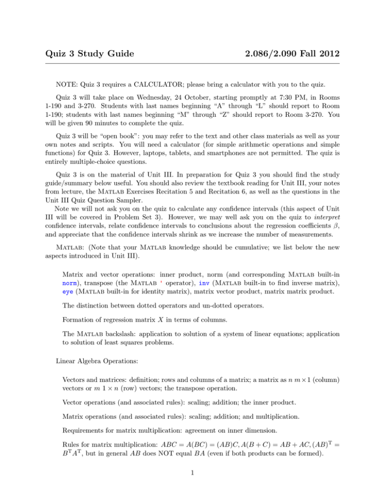
Quiz 3 Study Guide
2.086/2.090 Fall 2012
NOTE: Quiz 3 requires a CALCULATOR; please bring a calculator with you to the quiz.
Quiz 3 will take place on Wednesday, 24 October, starting promptly at 7:30 PM, in Rooms
1-190 and 3-270. Students with last names beginning “A” through “L” should report to Room
1-190; students with last names beginning “M” through “Z” should report to Room 3-270. You
will be given 90 minutes to complete the quiz.
Quiz 3 will be “open book”: you may refer to the text and other class materials as well as your
own notes and scripts. You will need a calculator (for simple arithmetic operations and simple
functions) for Quiz 3. However, laptops, tablets, and smartphones are not permitted. The quiz is
entirely multiple-choice questions.
Quiz 3 is on the material of Unit III. In preparation for Quiz 3 you should find the study
guide/summary below useful. You should also review the textbook reading for Unit III, your notes
from lecture, the Matlab Exercises Recitation 5 and Recitation 6, as well as the questions in the
Unit III Quiz Question Sampler.
Note we will not ask you on the quiz to calculate any confidence intervals (this aspect of Unit
III will be covered in Problem Set 3). However, we may well ask you on the quiz to interpret
confidence intervals, relate confidence intervals to conclusions about the regression coefficients β,
and appreciate that the confidence intervals shrink as we increase the number of measurements.
Matlab: (Note that your Matlab knowledge should be cumulative; we list below the new
aspects introduced in Unit III).
Matrix and vector operations: inner product, norm (and corresponding Matlab built-in
norm), transpose (the Matlab ' operator), inv (Matlab built-in to find inverse matrix),
eye (Matlab built-in for identity matrix), matrix vector product, matrix matrix product.
The distinction between dotted operators and un-dotted operators.
Formation of regression matrix X in terms of columns.
The Matlab backslash: application to solution of a system of linear equations; application
to solution of least squares problems.
Linear Algebra Operations:
Vectors and matrices: definition; rows and columns of a matrix; a matrix as n m × 1 (column)
vectors or m 1 × n (row) vectors; the transpose operation.
Vector operations (and associated rules): scaling; addition; the inner product.
Matrix operations (and associated rules): scaling; addition; and multiplication.
Requirements for matrix multiplication: agreement on inner dimension.
Rules for matrix multiplication: ABC = A(BC) = (AB)C, A(B + C) = AB + AC, (AB)T =
B T AT , but in general AB does NOT equal BA (even if both products can be formed).
1
Matrix vector products in terms of both the row interpretation (see page 222 of text) and the
column interpretation (page 223 of text).
Formulation of a system of m equations in n unknowns in terms of a matrix equation (e.g.,
Bz = g, for B an m × n matrix, z a n × 1 vector (the “unknown”), and g an m × 1 vector).
Definition of the identity matrix I. Definition of the inverse matrix for a non-singular matrix
A: A−1 A = AA−1 = I; formula for the inverse of a 2 × 2 non-singular matrix.
Suggestion: Practice vector and matrix operations “by hand” for small systems (e.g., for
matrix dimensions up to 2 × 3 and 3 × 2).
Least Squares and Regression:
The general model of Section 19.2.1: x, p, y, βj , hj , n, m; m×1 vector of measurements Y , and
m × n regression matrix X; fundamental relationship (Xβ)i = Ymodel (xi ; β), for i = 1, ..., m.
Notion of “bias-free” and β true . (We will only consider bias-free models in the quiz.) Con­
ditions for which Xβ = Y has a solution (i.e., when Y is noise free); conditions for which
Xβ = Y in general has no solution (i.e., when m > n and Y is noisy). Simple example of an
overdetermined system: a straight line through m > 2 points.
The residual vector r(β) = Y − Xβ as “misfit” or “misprediction”; the least squares formu­
lation — β̂ minimizes Ir(β)I2 over all possible β; the normal equations for β̂ — (X T X)β̂ =
X TY .
Assumptions on noise: normal and zero mean (N1); homoscedastic (N2) with standard devi­
ation σ (a scalar); uncorrelated (N3).
Regression estimates: estimate β̂ for β true ; estimate σ̂ (in terms of IY − Xβ̂I) for σ; “reason”
for m − n rather than just m in the σ̂ expression; interpretation of β̂ as “best explanation
of data” and of σ̂ as “what is left over”; joint confidence intervals for the β true in terms of
the n × n matrix Σ̂; frequentist interpretation of joint confidence intervals; “hypothesis test”
interpretation of joint confidence intervals (in particular, conclusions about coefficients β true );
shrinking of the confidence intervals as the number of measurements, m, increases.
Overfitting: why it is evil, why m should be large compared to n, and how overfitting is
reflected in confidence intervals.
2
MIT OpenCourseWare
http://ocw.mit.edu
2.086 Numerical Computation for Mechanical Engineers
Fall 2012
For information about citing these materials or our Terms of Use, visit: http://ocw.mit.edu/terms.