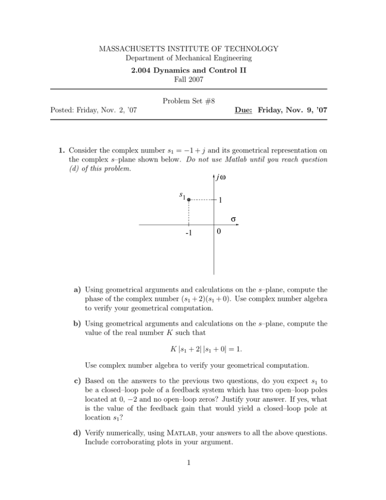
MASSACHUSETTS INSTITUTE OF TECHNOLOGY
Department of Mechanical Engineering
2.004 Dynamics and Control II
Fall 2007
Problem Set #8
Due: Friday, Nov. 9, ’07
Posted: Friday, Nov. 2, ’07
1. Consider the complex number s1 = −1 + j and its geometrical representation on
the complex s–plane shown below. Do not use Matlab until you reach question
(d) of this problem.
jω
s1
1
σ
-1
0
a) Using geometrical arguments and calculations on the s–plane, compute the
phase of the complex number (s1 + 2)(s1 + 0). Use complex number algebra
to verify your geometrical computation.
b) Using geometrical arguments and calculations on the s–plane, compute the
value of the real number K such that
K |s1 + 2| |s1 + 0| = 1.
Use complex number algebra to verify your geometrical computation.
c) Based on the answers to the previous two questions, do you expect s1 to
be a closed–loop pole of a feedback system which has two open–loop poles
located at 0, −2 and no open–loop zeros? Justify your answer. If yes, what
is the value of the feedback gain that would yield a closed–loop pole at
location s1 ?
d) Verify numerically, using Matlab, your answers to all the above questions.
Include corroborating plots in your argument.
1
2. Consider a feedback system with open–loop poles at 0, −1, −2 and no open–loop
zeros. The geometrical representation of this system’s open–loop poles on the
complex s–plane is shown below. Do not use Matlab until you reach question (f )
of this problem.
jω
2
σ
-2
-1
0
2
a) Using
√ geometrical arguments and calculations on the s–plane, show that
±j 2 belongs to the root locus of this system.
b) Using geometrical arguments and calculations on the s–plane, compute the
feedback gain K that would be√required to drive two closed–loop poles of
this system to the locations ±j 2.
c) Verify algebraically the results that you obtained geometrically in questions
(a–b).
d) What will happen to this system if K exceeds the value that you computed
in question (b)?
e) Sketch the complete root locus for this system. In your plot, indicate nu­
merical values for the asymptote angles and real–axis intercepts, as well as
the break–in/away points, if any.
f ) Verify numerically, using Matlab, your answers to all the above questions.
Include corroborating plots in your argument.
3. Consider a system with open–loop poles at −1, −2. Initially, this system is
connected in proportional control feedback configuration, with gain K. The
application where this system is to be used requires that the overshoot not exceed
16.3%. Do not use Matlab until you reach question (h) of this problem.
a) Sketch the root locus for this system.
b) Using geometrical arguments and calculations on the s–plane, find the closed–
loop pole location that will yield the desired overshoot. Do you expect your
answer to be exact or approximate?
2
c) What is the settling time at the closed–loop pole chosen from the previous
question?
d) Using geometrical arguments and calculations on the s–plane, compute the
value of the gain K that will drive the closed–loop pole to the location used
in the previous two questions.
e) We now wish to reduce the settling time to 75% of the value obtained in
question (c) while maintaining the same overshoot. Therefore, we propose to
modify the feedback loop from its present proportional–control configuration
to a proportional–derivative (PD) control configuration. Using geometrical
arguments and calculations on the s–plane, design the PD controller that
meets the new specifications (i.e., indicate where the open–loop zero should
be placed on the negative real axis.) Hint: Study and understand the PD
compensator design procedure described in Lecture 23 before you attempt
this question. The PD controller’s open–loop zero should be placed on the
real axis to the left of the existing open–loop pole at −2.
f ) Using geometrical arguments and calculations on the s–plane, compute the
PD controller’s gain that will result in the desired transient performance.
Do you expect that the settling time and overshoot requirements will be
met exactly or approximately in the new PD controller configuration?
g) Sketch the root locus of the PD–compensated system.
h) Verify numerically, using Matlab, your answers to all the above questions.
Include corroborating plots in your argument.
4. Given the matrices
3 1
A=
,
−1 3
and the vectors
p=
−1
1
B=
2 −1
3 5
,
q =
,
I=
e−3t cos t
e−3t sin t
1 0
0 1
,
compute the matrices sI − A, AB, B−1 A, and the vectors Bp, Aq. You should
study the auxiliary material on matrices that we have posted in the Stellar
website before you attempt this problem.
5. In this problem, we will generate a state–space representation for the compensated
2.004 Tower system. (Recall that in Lecture 24 we developed a simplified model
for the uncompensated tower; you should thoroughly familiarize yourself with
the Lecture 24 notes and the auxiliary notes on matrices before you attempt
this problem.) The model is shown in the figure on next page. The wind force
(disturbance) is denoted as w, and the actuator force is denoted as a, as in the
3
notes. Note that the actuator exerts equal but opposite forces on the tower and
slider.
a) Which forces are acting on the tower? Be particularly careful when you
include the force due to spring k2 , since the spring extension is the relative
displacement of the tower with respect to the slider. Similarly, be particu­
larly careful when you include the force due to damper b2 , since damping
is due to the relative velocity of the tower with respect to the slider. By
applying force balance, obtain an equation of motion for the tower.
b) Which forces are acting on the slider? Be careful with the spring and damper
forces for the same reasons quoted in the previous question. By applying
force balance, obtain an equation of motion for the slider.
c) Now define the tower displacement and velocity x1 , v1 , respectively, and
slider displacement and velocity x2 , v2 , respectively, as the state variables,
and the state vector
⎞ ⎛
⎞
⎛
x1
q1
⎜ q2 ⎟ ⎜ v1 ⎟
⎟ ⎜
⎟
q=⎜
⎝ q3 ⎠ ≡ ⎝ x 2 ⎠ .
q4
v2
Rewrite the tower’s and slider’s equations of motion in terms of the state
variables q1 , q2 , q3 , q4 .
d) Solve the tower’s equation of motion for q̇2 and the slider’s equation of
motion for q̇4 .
e) To the two equations that you obtained in the previous question append the
definitions q2 = q̇1 , q4 = q̇3 . Rewrite the resulting four equations in matrix
form, i.e. find the matrix A and vectors B, G such that
q̇(t) = Aq(t) + Ba(t) + Gw(t).
4
We will refer to B, G as actuation and disturbance vectors, respectively.
(Note that in multi–input systems B and G would actually be matrices;
hence, the uppercase letter notation.)
Do not substitute numbers in your final matrix expression; you will do that as part
of your Lab 7 assignment. Using the state–space representation that we obtained
here to minimize the tower’s displacement in response to an impulse disturbance
is the subject of the next few lectures and the rest of the Lab assignments.
5