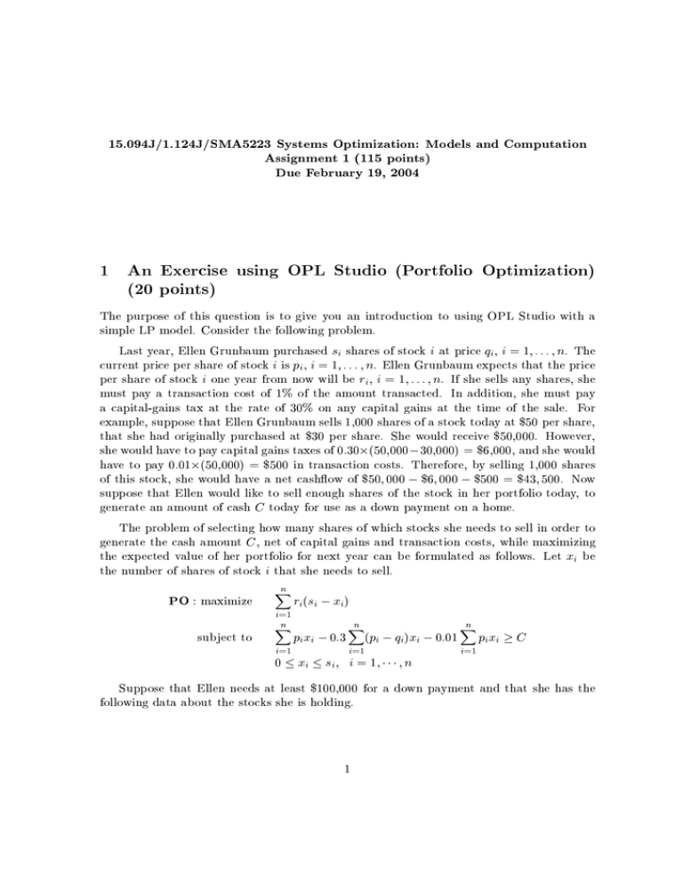
15.094J/1.124J/SMA5223 Systems Optimization: Models and Computation
Assignment 1 (115 p oints)
Due February 19, 2004
1
An Exercise using OPL Studio (Portfolio Optimization)
(20 p oints)
The purpose of this question is to give you an introduction to using OPL Studio with a
simple LP model. Consider the following problem.
Last year, Ellen Grunbaum purchased si shares of stock i at price qi , i = 1; : : : ; n. The
current price per share of stock i is pi , i = 1; : : : ; n. Ellen Grunbaum expects that the price
per share of stock i one year from now will be ri , i = 1; : : : ; n. If she sells any shares, she
must pay a transaction cost of 1% of the amount transacted. In addition, she must pay
a capital-gains tax at the rate of 30% on any capital gains at the time of the sale. For
example, suppose that Ellen Grunbaum sells 1,000 shares of a stock today at $50 per share,
that she had originally purchased at $30 per share. She would receive $50,000. However,
she would have to pay capital gains taxes of 0.30(50,000 30,000) = $6,000, and she would
have to pay 0.01(50,000) = $500 in transaction costs. Therefore, by selling 1,000 shares
of this stock, she would have a net cashow of $50; 000 $6; 000 $500 = $43; 500. Now
suppose that Ellen would like to sell enough shares of the stock in her portfolio today, to
generate an amount of cash C today for use as a down payment on a home.
The problem of selecting how many shares of which stocks she needs to sell in order to
generate the cash amount C , net of capital gains and transaction costs, while maximizing
the expected value of her portfolio for next year can be formulated as follows. Let xi be
the number of shares of stock i that she needs to sell.
PO
: maximize
subject to
Xn r (s
i i
xi )
i i
0:3
i=1
n
Xp x
i=1
Xn (p
i=1
i
qi )xi 0:01
0 xi si ; i = 1; ; n
Xn p x C
i i
i=1
Suppose that Ellen needs at least $100,000 for a down payment and that she has the
following data about the stocks she is holding.
1
Stocks i
1
2
3
4
5
6
7
8
9
10
Shares si
3,000 200 200 1,500 600 500 1,200 400 200 2,100
Initial prices qi
50
73 40
80 140 60
82
24 100
33
Current prices pi
70
60 42
65 160 60
57
50 102
45
Future prices ri
75
65 40
85 170 60
68
55 100
50
(a)
and portfolio.dat are an OPL model le and the data le for the
above optimization problem, respectively. Download and unzip the zip le Prob1.zip
from the assignment section and go over the codes and the data to understand how to
write an optimization model using OPL and how to associate a data le with a model
le. Now create a project le and run the model. What is the optimal objective value?
What is the optimal solution?
For MIT students using MIT Server, the following two commands will open OPL Studio.
(Please use SUN workstations. SGI machines do not support OPL Studio.)
portfolio.mod
% add oplstudio
% oplst &
If you need help in working with OPL Studio, contact the teaching assistant.
Also, you might want to look at online reference guides for OPL Studio.
P
(b) The PO model has one drawback: Suppose ni=1 (pi qi )xi is negative. This means
that Ellen has negative capital gains if she sells xi shares of stock i, i = 1; ; n. In
this case, Ellen should neither pay taxes nor receive tax savings. In order to reect
this, the PO model should be re-formulated as follows:
MPO
: maximize
subject to
X r (s
n
i=1
n
i i
xi )
i i
0:3 maxf
Xp x
i=1
Xn (p
i=1
i
qi)xi ; 0g 0:01
0 xi si ; i = 1; ; n
Xn p x C
i i
i=1
How would you modify MPO to convert it to a linear program? Modify portfolio.mod, solve it using OPL Studio, and report the optimal objective value and the
optimal solution. Does the optimal objective value increase or decrease? Why?
2
Radiation Therapy Model (40 points)
The purpose of this question is to give you more experience in using OPL Studio by solving a
relatively large-scale linear optimization model, using a variety of dierent solution methods,
and making some changes to the model in the process.
On the assignmen t section, you will nd the zip le Prob2.zip which
contains the following les:
2
regular5.mod This is the OPL model le for the \base case" radiation therapy model
small5.mod
discussed in the rst lecture of the course.
This is the \small" version of the radiation therapy model discussed in
the rst lecture of the course.
opl505.dat
This is the data le for the radiation therapy problem.
This is a C-program that is used to automatically allow the output of
the radiation therapy model to be turned into a \picture" that can be displayed in
MATLAB.
display5.c
BOUNDARY5.hlp This is a supplementary le that is used to produce visual images
of the model output.
Part I. Run the \base case" model and produce a picture of the optimal solution. In order
to do so, proceed as follows:
First, download all les from the assignment section. Then open OPL Studio.
Prior to running the model, click the \Options" menu and the \Customize Active
Project Options" submenu. Change the project options in the following four ways:
Next, create a new project using the model le
opl505.dat.
{
{
{
{
regular5.mod
and the data le
(i) Under \MP General", change the \LP Method" to \Primal"
(ii) Under \Simplex", change \Pricing candidate list size" to 200
(iii) Under \Simplex", turn \Perturbation" to the on position.
(iv) Under \Preprocessing", change \Simplication with pre-solve" to the o
position.
Now you are ready to solve your optimization model. Do so by clicking the green Run
button.
After the model is solved, you will need to save the solution. First, click the green
\proceed" button. Then choose the \File" menu, and choose the \Dump Active Model
and Result . . . " submenu. Give your solution le a name such as \coolmodel.out".
In order to create a picture of the model output, compile the program display5.c
using the MIT Server commands add gnu and gcc display5.c. This will create the
executable le a.out. Execute this le by typing the command a.out . You will next
be prompted to supply an input le, for which you should type your model solution
output le coolmodel.out (or whatever name you called your output le). You will
need to specify the name of the new output le, such as \hotmodel" without an
extension.
3
Now you can open MATLAB by typing the commands add matlab and matlab.
Once MATLAB is open, type the commands load hotmodel and pcolor(hotmodel).
MATLAB will produce and display a picture of the optimal solution of the radiation
therapy model.
Part II. Experiment with the \base case" and \small" versions of the radiation therapy
model. Run the models regular5.mod and small5.mod using the two dierent LP methods \Primal" (which is the primal simplex algorithm) and \Barrier" (which is the interiorpoint logarithmic barrier algorithm described in the second lecture of the course). These
solution method options can be found in OPL Studio under \Options" then \Customize
Active Project Options" then \MP General". Fill in the following table:
Number
Number Running Number
of
of
time
of
Constraints Variables (seconds) Iterations
MODEL
Base Case
Algorithm
Primal Simplex
Barrier
Small Model Primal Simplex
Barrier
Part III. Experiment with dierent versions of the model to see if you can produce solutions
that look \better" to you. Here are two ideas for dierent versions of the model:
Idea #1. You might want to change the weights on the dierent pixel regions (T ,
C and N ) in the objective function, to see if you can produce better solutions. Try
to weight more on the tumor part and the critical part, respectively, and see what
happens.
Idea #2. In the rst lecture, you were shown several dierent linear optimization
models for this problem. In one of those models, the objective function was to minimize the maximum dierence between the delivered dose and target dose at each
pixel. This model was:
minimize
w;D;
s:t:
Dij
(Target)ij
Dij =
Xn Dp w
p=1
w0
4
ij
p
(i; j ) 2 S
(i; j ) 2 S
With slight changes, you can modify the given model les to become a version of this
formulation. How does your solution change? Is it better than any other of your solutions?
If you have any questions about the model, please send an email to the MIT Teaching
Assistant .
3
Variable Upper and Lower Bounds (20 points)
Consider the general linear programming problem with upper and lower bounds as follows:
LP : minimize z = cT x
Ax = b
lxu:
s.t.
Suppose that the simplex tableau for such an instance of this problem is as shown in
Table 1. Answer the following questions:
UB
LB
RHS
7
11
25
20
3
0
8
1
10
2
8
1
6
2
10
1
x1 x2 x3
x4
x5
x6
0
1
0
0
0
0
1
0
0
0
0
1
1
3
3
2
5
3
4
5
4
6
5
2
Table 1: A simplex tableau.
1. What is the basic solution corresponding to the tableau in Table 1? Why is this
solution feasible?
2. Why is this basic solution also optimal?
3. Suppose that the tableau objective coeÆcient on x4 is changed from 1 to 1. Then
the tableau would look like that shown in Table 2. What would be the next change in
the basis for this tableau that would improve the objective function value? Compute
the next tableau.
4. Now suppose that the lower bound on x4 is changed from 0 to 2. Then the tableau
would like that shown in Table 3. What would be the next change in the basis for this
tableau that would improve the objective function value? Compute the next tableau.
5
UB
LB
RHS
7
11
25
20
8
1
10
2
8
1
3
0
x1 x2 x3 x4
x5
x6
0
1
0
0
0
0
1
0
0
0
0
1
1
3
3
2
5
3
4
5
4
6
5
2
6
2
10
1
Table 2: Another simplex tableau.
UB
LB
RHS
7
11
25
20
8
1
10
2
8
1
3
2
x1 x2 x3 x4
x5
x6
0
1
0
0
0
0
1
0
0
0
0
1
1
3
3
2
5
3
4
5
4
6
5
2
6
2
10
1
Table 3: A third simplex tableau.
4
Lagrange Duality Problems (20 points)
A. Construct a Lagrange dual of the following problem:
BP43 : minimumx;s cT x
43
Pm ln sj
i=1
Ax + s = b
s>0
s.t.
B. Consider the following problem:
P : minimizex;y cT x
s.t.
Gx
Nx + My
y binary integer
f
d
It is helpful in this problem to think of the variables x as production decisions and the
binary integer variables y as set-up decisions. The constraints \Gx f " are ordinary
resource and/or capacity constraints on the production levels x, and the constraints
\Nx + My d" can be thought of as arising from the eects of set-up decisions y on
the production activities x.
6
x0
d
(5; 7)
(1; 2)
( 30; 50) (1; 1)
(20; 10) ( 1; 0)
u
2:3
1:5
5:6
Table 4: Starting points, directions, and step-size upper bound.
(a)
(b)
(c)
5
Construct a \good" dual of this problem. What makes your choice of dual
problem \good"?
For a given value of your dual variables u, how would you solve for the value of
L (u)?
What type of algorithm might you use to solve the dual problem?
Bisection Line-Search Algorithm (15 points)
Consider the function:
f (x) = 25 4x1 6x2 + (3x1 6x2 10)2 + (x1 + x2 + 15)2
+(x1 x2 + 4)4 + 101 (5x1 + x2 6)6 :
Given a current point x0 = (x01 ; x02 ) and a direction d = (d1 ; d2 ), we are interested in
solving the 1-dimensional minimization problem:
P:
min h() := f (x0 + d)
Construct a bisection algorithm, coded either in OPLScript or Matlab, to solve this
problem. The algorithm should be designed to take as input a starting point x0 , a
direction d, and an initial value for the upper bound u . Be certain to specify a
stopping criteria for your algorithm. Your code should check whether or not d is a
descent direction (and terminate if it is not), and should check that u is a valid upper
bound on the optimal step-size .
Solve for the minimizing value of using your algorithm for the three problem instances shown in Table 4.
Hand in a hard copy of your code.
7