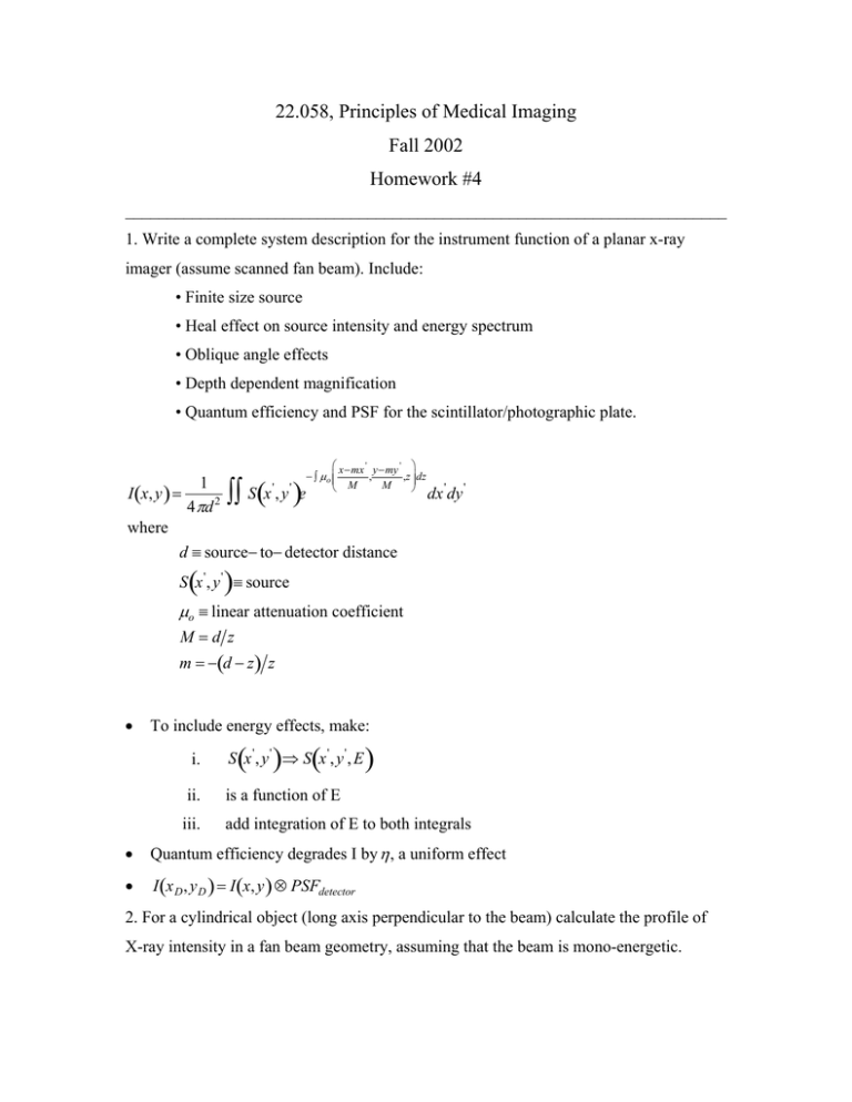
22.058, Principles of Medical Imaging Fall 2002 Homework #4 ________________________________________________________________________ 1. Write a complete system description for the instrument function of a planar x-ray
imager (assume scanned fan beam). Include:
• Finite size source
• Heal effect on source intensity and energy spectrum
• Oblique angle effects
• Depth dependent magnification
• Quantum efficiency and PSF for the scintillator/photographic plate.
 x−mx ' y−my ' 
,z  dz

− ∫ µ o 
,
1
M
' '
 M
S
x
,
y
e
I (x, y ) =
2
4 πd
where
d ≡ source− to− detector distance
∫∫ ( )
dx ' dy '
( )
S x ' , y ' ≡ source
µo ≡ linear attenuation coefficient
M=d z
m = −(d − z) z
• To include energy effects, make:
•
( )
(
)
i.
S x ', y ' ⇒ S x ', y ', E
ii.
is a function of E
iii.
add integration of E to both integrals
Quantum efficiency degrades I by η , a uniform effect
• I (x D , y D ) = I (x, y ) ⊗ PSFdetector
2. For a cylindrical object (long axis perpendicular to the beam) calculate the profile of
X-ray intensity in a fan beam geometry, assuming that the beam is mono-energetic.
QuickTime™ and a
None decompressor
are needed to see this picture.
1, if (z − a)2 + x 2 ≤ r
µ(x,z) = 
0, otherwise
1
I (x ) =
4 πd 2
M=
∫e
 x−mx ' 
− ∫ µ 
,z  dz
 M

dx '
−(d − z )
d
and m =
z
z
  d − z '
z x + 
x 
x − mx
z
  z   zx
∴
=
= + x' − x'
M
d
d
d
'
1
I (x ) =
4 πd 2
∫e
z

− ∫ µ  x−x ' +x '  dz
d

( )
dx '
3. Calculate the effect of beam hardening on the CT image of a disk.
The center is less attenuating than it should be, therefore the image is:
QuickTime™ and a
None decompressor
are needed to see this picture.
4. For the following sample, show (a) the projections and (b) the filtered projections.
QuickTime™ and a
None decompressor
are needed to see this picture.
See Appendix A.
5. A sinusoidally modulated x-ray image is recorded by a one-sided screen film system as
shown below. Find the recorded S/N as a function of frequency, where the signal is the
sinusoidal component and the noise is the average background. On average the screen
produces l photons per x-ray photon, t of which are transmitted to the emulsion where r is
recorded. The pixel area of the film is much smaller than the system resolution. Neglect
any critical angle effect between the screen and the film.
X-ray photon number as a function of z = n0 (1+cos(2 π k z)).
QuickTime™ and a
None decompressor
are needed to see this picture.
d
PSF =
M
∫
e−µx r
2
dx
0
or in 1− D
d
PSF =
M
∫
e−µx z
0
2
dx
6. Write a program that calculates the Radon transform of an object function, then Fourier
filters the projects, and finally reconstructs an image via back projection.
See Appendix A.
APPENDIX A: Mathematica File (Projection2.nb)
Projection reconstruction and the Radon Transform 2
The Radon Transform
The forward Radon transform is to convert a 2-D object into a set of projects within the
plane.
Radon[object_, n_, fov_] := Table [ Integrate [ object DiracDelta [ m - x Cos[\[Theta]] - y Sin[\[Theta]] ], {x, -fov, fov}, {y, -fov, fov} ], {m, -2 fov/(n - 1), +2 fov/(n - 1), 2 fov/n}, {\[Theta], 0, Pi, Pi/(n - 1)} ];
The double integral on the previous page is very slow to evaluate, and so we reduce it to
a line integral along the line defined by the delta function.
Radon2[object_, x_, y_, n_, fov_] := Table [ Nintegrate [ object[x, y], {yp, -fov, fov}, {PrecisionGoal -> 4} ], {xp, -fov, fov, 2*fov/(n - 1)}, {\[Theta], 0, Pi, Pi/(n - 1)} ] // N Define a simple test object
object1[x_, y_] := If[x^2 + y^2 < 256, 1, 10^(-6)] // N; Plot3D [ object1[x, y], {x, -64, 64}, {y, -64, 64}, {PlotRange -> All, PlotPoints -> {64, 64}} ] Robject1 = Radon2 [ object1, xp Cos[\[Theta]] - yp Sin[\[Theta]], yp Cos[\[Theta]] + xp Sin[\[Theta]], 64, 64 ];
ListPlot3D[Robject1] Filtered Back Projection
Fdata = Fourier[Robject1]; ListPlot3D[Re[Fdata], {PlotRange -> All}] Filt = Table [ If [ x <= 32 && y <= 32, Sqrt[x^2 + y^2], If [ x <= 32 && y > 32, Sqrt[x^2 + (65 - y)^2], If [ x > 32 && y <= 32, Sqrt[(65 - x)^2 + y^2], If [ x > 32 && y > 32, Sqrt[(65 - x)^2 + (65 - y)^2] ] ] ] ], {x, 0, 63}, {y, 0, 63} ]; ListPlot3D[Filt] FiltFdata = Fdata*Filt;
ListPlot3D[Re[FiltFdata], {PlotRange -> All}]
Filtdata = Fourier[FiltFdata]; ListPlot3D[Re[Filtdata], {PlotRange -> All}] Back Projection of Filtered
Bflimited[x_, y_, n_] := If [ x^2 + y^2 > 32^2, 0, 1/(2 Pi) Sum [ Transpose [ Re[Filtdata] ] [[m*64 + 1]] [[Floor[x Cos[m*Pi] + y Sin[m Pi]] + 33]], {m, 0, 1 - 1/n, 1/n} ] ]; Plot3D [ BFlimited[x, y, 4], {x, -32, 32}, {y, -32, 32}, {PlotRange -> All, PlotPoints -> {64, 64}} ] DensityPlot [ BFlimited[x, y, 4], {x, -32, 32}, {y, -32, 32}, {PlotRange -> All, PlotPoints -> {64, 64}, Mesh -> False} ] Image = Table [ BFlimited[x, y, 64], {x, -32, 32}, {y, -32, 32} ]; ListPlot3D[Image, {PlotRange -> All}] ListDensityPlot[Image, {PlotRange -> {0, 500}, Mesh -> False}]