6.042/18.062J Mathematics for Computer Science
Srini Devadas and Eric Lehman
May 6, 2005
Notes for Recitation 22
1 Conditional Expectation and Total Expectation
There are conditional expectations, just as there are conditional probabilities. If R is a
random variable and E is an event, then the conditional expectation Ex (R | E) is defined
by:
�
Ex (R | E) =
R(w) · Pr (w | E)
w∈S
For example, let R be the number that comes up on a roll of a fair die, and let E be the
event that the number is even. Let’s compute Ex (R | E), the expected value of a die roll,
given that the result is even.
�
Ex (R | E) =
R(w) · Pr (w | E)
w∈{1,...,6}
=1·0+2·
1
1
1
+3·0+4· +5·0+6·
3
3
3
=4
It helps to note that the conditional expectation, Ex (R | E) is simply the expectation of
R with respect to the probability measure PrE () defined in PSet 10. So it’s linear:
Ex (R1 + R2 | E) = Ex (R1 | E) + Ex (R2 | E) .
Conditional expectation is really useful for breaking down the calculation of an ex­
pectation into cases. The breakdown is justified by an analogue to the Total Probability
Theorem:
Theorem 1 (Total Expectation). Let E1 , . . . , En be events that partition the sample space and
all have nonzero probabilities. If R is a random variable, then:
Ex (R) = Ex (R | E1 ) · Pr (E1 ) + · · · + Ex (R | En ) · Pr (En )
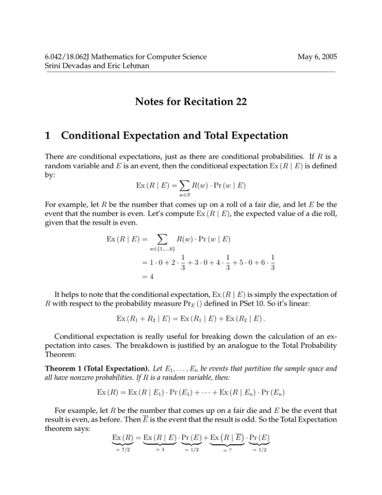
For example, let R be the number that comes up on a fair die and E be the event that
result is even, as before. Then E is the event that the result is odd. So the Total Expectation
theorem says:
�
�
Ex (R) = Ex (R | E) · Pr (E) + Ex R | E · Pr (E)
� �� � � �� � � �� � � �� � � �� �
= 7/2
=4
= 1/2
=?
= 1/2
Recitation 22
2
�
�
The only quantity here that we don’t already know is Ex R | E , which is the expected
die roll,�given �that the result is odd. Solving this equation for this unknown, we conclude
that Ex R | E = 3.
To prove the Total Expectation Theorem, we begin with a Lemma.
Lemma. Let R be a random variable, E be an event with positive probability, and IE be the
indicator variable for E. Then
Ex (R | E) =
Ex (R · IE )
Pr (E)
(1)
Proof. Note that for any outcome, s, in the sample space,
�
0
if IE (s) = 0,
Pr ({s} ∩ E) =
Pr (s) if IE (s) = 1,
and so
Pr ({s} ∩ E) = IE (s) · Pr (s) .
(2)
Now,
Ex (R | E) =
�
R(s) · Pr ({s} | E)
(Def of Ex (· | E))
s∈S
=
�
=
�
R(s) ·
Pr ({s} ∩ E)
Pr (E)
(Def of Pr (· | E))
R(s) ·
IE (s) · Pr (s)
Pr (E)
(by (2))
s∈S
s∈S
�
· IE (s)) · Pr (s)
Pr (E)
Ex (R · IE )
=
Pr (E)
=
s∈S (R(s)
(Def of Ex (R · IE ))
Now we prove the Total Expectation Theorem:
Proof. Since the Ei ’s partition the sample space,
�
R=
R · IEi
i
(3)
Recitation 22
3
for any random variable, R. So
�
�
�
R · IEi
Ex (R) = Ex
(by (3))
i
=
�
=
�
Ex (R · IEi )
(linearity of Ex ())
i
i
Ex (R | Ei ) · Pr (Ei )
(by (1))
Recitation 22
4
Problem 1. Final exams in 6.042 are graded according to a rigorous procedure:
• With probability 47 the exam is graded by a recitation instructor, with probability 72 it
is graded by a lecturer, and with probability 71 , it is accidentally dropped behind the
radiator and arbitrarily given a score of 84.
• Recitation instructors score an exam by scoring each problem individually and then
taking the sum.
– There are ten true/false questions worth 2 points each. For each, full credit is
given with probability 43 , and no credit is given with probability 14 .
– There are four questions worth 15 points each. For each, the score is deter­
mined by rolling two fair dice, summing the results, and adding 3.
– The single 20 point question is awarded either 12 or 18 points with equal prob­
ability.
• Lecturers score an exam by rolling a fair die twice, multiplying the results, and then
adding a “general impression” score.
– With probability
– With probability
– With probability
4
,
10
3
,
10
3
,
10
the general impression score is 40.
the general impression score is 50.
the general impression score is 60.
Assume all random choices during the grading process are mutually independent.
(a) What is the expected score on an exam graded by a recitation instructor?
Solution. Let X equal the exam score and C be the event that the exam is graded by
a recitation instructor. We want to calculate Ex (X | C). By linearity of (conditional)
expectation, the expected sum of the problem scores is the sum of the expected
problem scores. Therefore, we have:
Ex (X | C) = 10 · Ex (T/F score | C) + 4 · Ex (15pt prob score | C) + Ex (20pt prob score | C)
�
�
�
� �
�
3
1
7
1
1
·2+ ·0 +4· 2· +3 +
· 12 + · 18
= 10 ·
4
4
2
2
2
3
= 10 · + 4 · 10 + 15 = 70
2
(b) What is the expected score on an exam graded by a lecturer?
Recitation 22
5
�
�
Solution. Now we want Ex X | C¯ , the expected score a lecturer would give.
Employing linearity again, we have:
�
�
�
�
Ex X | C¯ = Ex product of dice | C¯
�
�
+ Ex general impression | C¯
� �2
7
=
(because the dice are independent)
2
�
�
4
3
3
+
· 40 +
· 50 +
·
60
10
10
10
49
1
=
+ 49 = 61
4
4
(c) What is the expected score on a 6.042 exam?
Solution. Let X equal the true exam score. The Total Expectation Theorem implies:
�
� � �
Ex (X) = Ex (X | C) Pr (C) + Ex X | C¯ Pr C¯
�
�
4
49
2
1
= 70 · +
+ 49 · + 84 ·
7
4
7
7
�
�
7
1
= 40 +
+ 14 + 12 = 69
2
2
Recitation 22
6
Problem 2. Here’s yet another fun 6.042 game! You pick a number between 1 and 6. Then
you roll three fair, independent dice.
• If your number never comes up, then you lose a dollar.
• If your number comes up once, then you win a dollar.
• If your number comes up twice, then you win two dollars.
• If your number comes up three times, you win four dollars!
What is your expected payoff? Is playing this game likely to be profitable for you or not?
Solution. Let the random variable R be the amount of money won or lost by the player
in a round. We can compute the expected value of R as follows:
Ex (R) = −1 · Pr (0 matches) + 1 · Pr (1 match) + 2 · Pr (2 matches) + 4 · Pr (3 matches)
� � � �2
� �2 � �
� �3
� �3
5
1
5
1
5
1
+1·3
+2·3
+4·
= −1 ·
6
6
6
6
6
6
−125 + 75 + 30 + 4
=
216
−16
=
216
You can expect to lose 16/216 of a dollar (about 7.4 cents) in every round. This is a horrible
game!
Recitation 22
7
Problem 3. The number of squares that a piece advances in one turn of the game Monopoly
is determined as follows:
• Roll two dice, take the sum of the numbers that come up, and advance that number
of squares.
• If you roll doubles (that is, the same number comes up on both dice), then you roll a
second time, take the sum, and advance that number of additional squares.
• If you roll doubles a second time, then you roll a third time, take the sum, and
advance that number of additional squares.
• However, as a special case, if you roll doubles a third time, then you go to jail.
Regard this as advancing zero squares overall for the turn.
(a) What is the expected sum of two dice, given that the same number comes up on
both?
Solution. There are six equally­probable sums: 2, 4, 6, 8, 10, and 12. Therefore, the
expected sum is:
1
1
1
· 2 + · 4 + . . . + · 12 = 7
6
6
6
(b) What is the expected sum of two dice, given that different numbers come up? (Use
your previous answer and the Total Expectation Theorem.)
Solution. Let the random variables D1 and D2 be the numbers that come up on the
two dice. Let E be the event that they are equal. The Total Expectation Theorem
says:
�
�
� �
Ex (D1 + D2 ) = Ex (D1 + D2 | E) · Pr (E) + Ex D2 + D2 |E · Pr E
Two dice are equal with probability Pr (E) = 1/6, the expected sum of two indepen­
dent dice is 7, and we just showed that Ex (D1 + D2 | E) = 7. Substituting in these
quantities and solving the equation, we find:
�
� 5
1
7 = 7 · + Ex D2 + D2 | E ·
6
6
�
�
Ex D2 + D2 | E = 7
(c) To simplify the analysis, suppose that we always roll the dice three times, but may
ignore the second or third rolls if we didn’t previously get doubles. Let the random
variable Xi be the sum of the dice on the i­th roll, and let Ei be the event that the
i­th roll is doubles. Write the expected number of squares a piece advances in these
terms.
Recitation 22
8
Solution. From the total expectation formula, we get:
�
�
� �
Ex (advance) = Ex X1 | E1 · Pr E1
�
�
�
�
+ Ex X1 + X2 | E1 ∩ E2 · Pr E1 ∩ E2
�
�
�
�
+ Ex X1 + X2 + X3 | E1 ∩ E2 ∩ E3 · Pr E1 ∩ E2 ∩ E3
+ Ex (0 | E1 ∩ E2 ∩ E3 ) · Pr (E1 ∩ E2 ∩ E3 )
Then using linearity of (conditional) expectation, we refine this to
Ex (advance)
�
�
� �
= Ex X1 | E1 · Pr E1
� �
�
�
��
�
�
+ Ex X1 | E1 ∩ E2 + Ex X2 | E1 ∩ E2 · Pr E1 ∩ E2
� �
�
�
�
�
��
+ Ex X1 | E1 ∩ E2 ∩ E3 + Ex X2 | E1 ∩ E2 ∩ E3 + Ex X3 | E1 ∩ E2 ∩ E3
�
�
·
Pr E1 ∩ E2 ∩ E3
+ 0.
Using mutual independence of the rolls, we simplify this to
Ex (advance)
�
�
� �
= Ex X1 | E1 · Pr E1
(4)
�
�
��
� �
+ Ex (X1 | E1 ) + Ex X2 | E2 · Pr (E1 ) · Pr E2
�
�
��
� �
+ Ex (X1 | E1 ) + Ex (X2 | E2 ) + Ex X3 | E3 · Pr (E1 ) · Pr (E2 ) · Pr E3
(d) What is the expected number of squares that a piece advances in Monopoly?
Solution. We plug the values from parts (a) and (b) into equation (4):
5
1 5
1 1 5
+ (7 + 7) · · + (7 + 7 + 7) · · ·
6
6 6
6 6 6
19
=8
72
Ex (advance) = 7 ·