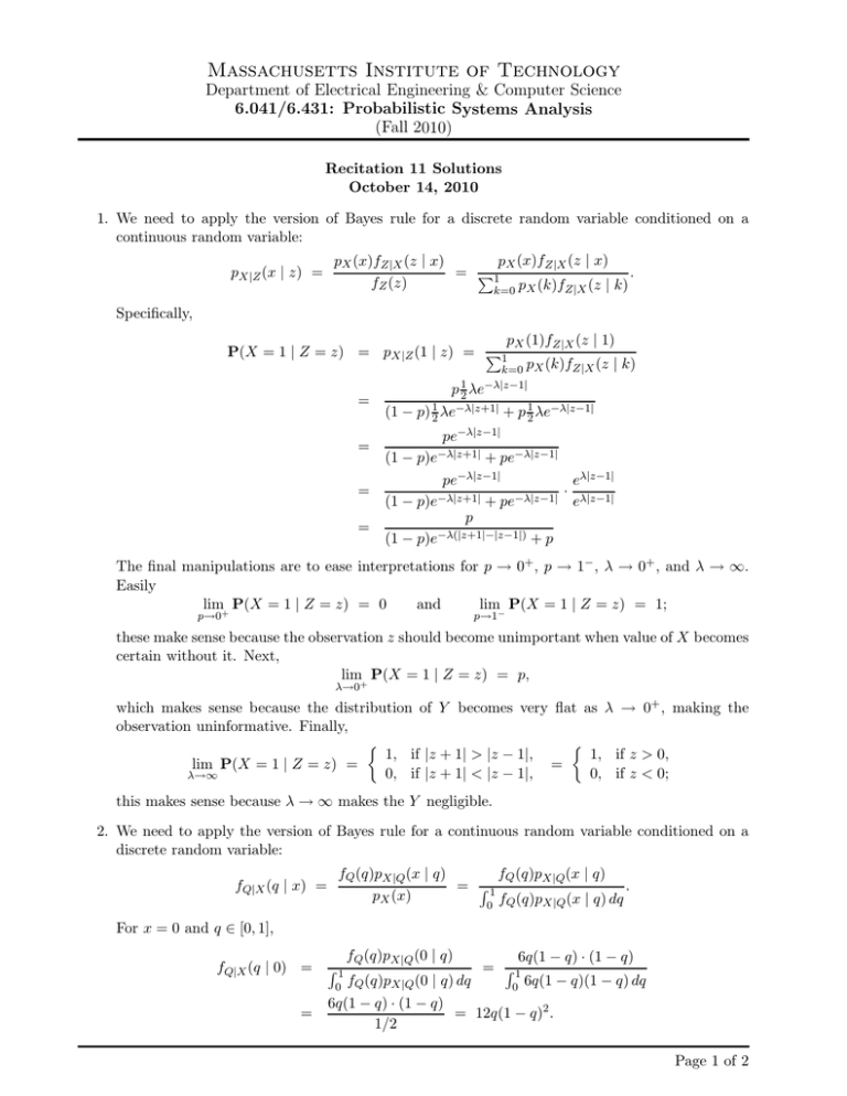
Massachusetts Institute of Technology
Department of Electrical Engineering & Computer Science
6.041/6.431: Probabilistic Systems Analysis
(Fall 2010)
Recitation 11 Solutions
October 14, 2010
1. We need to apply the version of Bayes rule for a discrete random variable conditioned on a
continuous random variable:
pX|Z (x | z) =
Specifically,
pX (x)fZ|X (z | x)
pX (x)fZ|X (z | x)
.
= �1
fZ (z)
k =0 pX (k)fZ|X (z | k)
pX (1)fZ|X (z | 1)
P(X = 1 | Z = z) = pX|Z (1 | z) = �1
k=0 pX (k)fZ|X (z | k)
=
=
=
=
p 12 λe−λ|z−1|
(1 − p) 21 λe−λ|z+1| + p 12 λe−λ|z−1|
pe−λ|z−1|
(1 − p)e−λ|z+1| + pe−λ|z−1|
pe−λ|z−1|
eλ|z−1|
·
(1 − p)e−λ|z+1| + pe−λ|z−1| eλ|z−1|
p
−λ(|z+1|−|z−1|)
+p
(1 − p)e
The final manipulations are to ease interpretations for p → 0+ , p → 1− , λ → 0+ , and λ → ∞.
Easily
lim P(X = 1 | Z = z) = 0
and
lim P(X = 1 | Z = z) = 1;
p→0+
p→1−
these make sense because the observation z should become unimportant when value of X becomes
certain without it. Next,
lim P(X = 1 | Z = z) = p,
λ→0+
which makes sense because the distribution of Y becomes very flat as λ → 0+ , making the
observation uninformative. Finally,
�
�
1, if |z + 1| > |z − 1|,
1, if z > 0,
lim P(X = 1 | Z = z) =
=
0, if |z + 1| < |z − 1|,
0, if z < 0;
λ→∞
this makes sense because λ → ∞ makes the Y negligible.
2. We need to apply the version of Bayes rule for a continuous random variable conditioned on a
discrete random variable:
fQ|X (q | x) =
For x = 0 and q ∈ [0, 1],
fQ|X (q | 0) =
=
fQ (q)pX|Q (x | q)
fQ (q)pX|Q (x | q)
= �1
.
pX (x)
f
(q)p
(x
|
q)
dq
Q
X|Q
0
fQ (q)pX|Q (0 | q)
6q(1 − q) · (1 − q)
= �1
0 fQ (q)pX|Q (0 | q) dq
0 6q(1 − q)(1 − q) dq
6q(1 − q) · (1 − q)
= 12q(1 − q)2 .
1/2
�1
Page 1 of 2
Massachusetts Institute of Technology
Department of Electrical Engineering & Computer Science
6.041/6.431: Probabilistic Systems Analysis
(Fall 2010)
For x = 1 and q ∈ [0, 1],
fQ|X (q | 1) =
=
�1
0
fQ (q)pX|Q (1 | q)
6q(1 − q) · q
= �1
fQ (q)pX|Q (1 | q) dq
0 6q(1 − q)q dq
6q(1 − q) · q
= 12q 2 (1 − q).
1/2
The distributions fQ (q), fQ|X (q | 0), and fQ|X (q | 1) are all in the family of beta distributions,
which arise again in Chapter 8.
3. Because of the definition of g, the random variable Y takes on only nonnegative values. Thus
fY (y) = 0 for any negative y. For y > 0,
FY (y) = P(Y ≤ y)
�
�
= P (X ∈ [−y, 0]) + P X ∈ (0, y 2 ]
�
�
= (FX (0) − FX (−y)) + FX (y 2 ) − FX (0)
= FX (y 2 ) − FX (−y).
Taking the derivative of FY (y) (and using the chain rule),
fY (y) = 2yfX (y 2 ) + fX (−y)
�
2
1 � −y4 /2
= √
2ye
+ e−y /2 .
2π
Page 2 of 2
MIT OpenCourseWare
http://ocw.mit.edu
6.041SC Probabilistic Systems Analysis and Applied Probability
Fall 2013
For information about citing these materials or our Terms of Use, visit: http://ocw.mit.edu/terms.