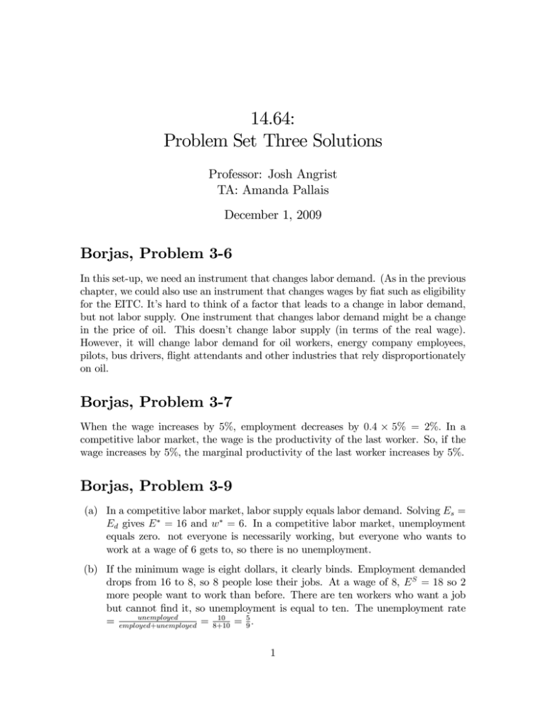
14.64:
Problem Set Three Solutions
Professor: Josh Angrist
TA: Amanda Pallais
December 1, 2009
Borjas, Problem 3-6
In this set-up, we need an instrument that changes labor demand. (As in the previous
chapter, we could also use an instrument that changes wages by …at such as eligibility
for the EITC. It’s hard to think of a factor that leads to a change in labor demand,
but not labor supply. One instrument that changes labor demand might be a change
in the price of oil. This doesn’t change labor supply (in terms of the real wage).
However, it will change labor demand for oil workers, energy company employees,
pilots, bus drivers, ‡ight attendants and other industries that rely disproportionately
on oil.
Borjas, Problem 3-7
When the wage increases by 5%, employment decreases by 0:4 5% = 2%: In a
competitive labor market, the wage is the productivity of the last worker. So, if the
wage increases by 5%, the marginal productivity of the last worker increases by 5%.
Borjas, Problem 3-9
(a) In a competitive labor market, labor supply equals labor demand. Solving Es =
Ed gives E = 16 and w = 6. In a competitive labor market, unemployment
equals zero. not everyone is necessarily working, but everyone who wants to
work at a wage of 6 gets to, so there is no unemployment.
(b) If the minimum wage is eight dollars, it clearly binds. Employment demanded
drops from 16 to 8, so 8 people lose their jobs. At a wage of 8, E S = 18 so 2
more people want to work than before. There are ten workers who want a job
but cannot …nd it, so unemployment is equal to ten. The unemployment rate
unemployed
10
= 8+10
= 59 :
= employed+unemployed
1
Borjas, Problem 3-12
The higher the elasticity of labor demand, the more labor demand decreases when
the wage increases. thus, the minimum wage will lead to more unemployment when
there is a high elasticity of labor demand. I would think that labor demand is more
elastic in the lawn-care industry than in the fast-food industry. When the price of
lawn-care workers increases, consumers have more options that didn’t face the same
increase in price. They can hire a neighbor who is not subject to the minimum wage
to cut their grass, hire an illegal immigrant (many of whom work in these types of
industries in the West) or do it themselves. Consumers in a fast food restaurant may
not be as elastic in their demand, so that the labor demanded for fast food workers
might not fall as much in response to an increase in wages. Thus, employment in the
minimum wage would have a greater e¤ect in the lawn-care industry.
Borjas, Problem 4-5
(a) Remember that labor and wages are jointly determined by the monopsonist
with
pf 0 (L) = w(L)[1 + ]:
If there exists a payroll tax then we must replace w(L) with
w(L), where
> 1 is some factor that adjusts for the fact that the monopsonist will have to
pay higher wages now. (Who bears all of the tax is a seperate question.) This
leads to a lower equilibrium wage and employment overall. In the monopsony
graph we always stare at, this means that the w(L) curve shifts even farther
left.
In a perfectly competitive labor market, the demand curve will shift in as a result
of the tax, leading to lower wages and employment, as well. But remember that
the competitive market had a higher level of employment to begin with.
(b) A perfectly discriminating monopsonist is a monopsonist that can pay each of
his workers a di¤erent wage. He will hire the perfectly competitive number
of workers, because the perfectly discriminating monopsonist does not have to
worry about how the marginal worker’s wage a¤ects the wages of the inframarginal workers. Consequently, the minimum wage would lower employment (if it
binds) and raise average wages.
Borjas, Problem 4-10
(a) If Ann uses push mowers, each laborer will take two hours to cut each lawn. So
she will have to demand 400 2 = 800 hours of labor. That’s a total labor cost
of 5 800 = 4000 dollars. Each worker can supply a total of 8 5 = 40 hours
of labor a week, so she would need 20 workers and 20 push mowers.
2
(b) If Ann uses riding mowers, each laborer will take half an hour to cut each lawn.
So she will have to demand 400 12 = 200 hours. Each worker can supply 40
hours of labor, so she would only need …ve laborers and …ve riding mowers.
That’s a total labor bill of 5 200 = 1000 dollars.
(c) We can compare total costs under the two technologies. Using push mowers,
her total costs are 250 20 + 5 20 40 = 9000. Using riding mowers, her
total costs are 1800 5 + 5 5 40 = 10000. So she’ll use the less e¢ cient
technology, push mowers.
(d) The costs for the push mowers are now (250(1 0:2)) 20+(5(1+0:2)) 40 20 =
8800. The costs for riding mowers are now (1800(1 0:2)) 5 + (5(1 + 0:2))
20 40 = 8400. So Ann will now switch to the more advanced technology.
Borjas, Problem 6-1
(a) If the interest rate is 5%, then in period 2 dollars Debbie earns
15; 000
1:05 + 472; 000 = 456; 250 as a marine biologist and
40; 000
1:05 + 500; 000 = 458; 000 as a concert pianist.
So she will choose to be a concert pianist.
If the interest rate is 15%, then in period 2 dollars Debbie earns
15; 000
1:15 + 472; 000 = 454; 750 as a marine biologist and
40; 000
1:15 + 500; 000 = 454; 000 as a concert pianist.
So she will choose to be a marine biologist. The higher rate of interest means
that from the standpoint of period 2 schooling costs incurred in period 1 become
more expensive, so now the option with the lower schooling costs (and lower
salary) becomes more attractive.
(b) Under this scenario in period 2 dollars, Debbie earns
15; 000
1:05 + 472; 000 = 456; 250 as a marine biologist and
60; 000
1:05 + 500; 000 = 437; 000 as a concert pianist.
So she will choose to be a marine biologist.
1
Borjas, Problem 6-2
If Peter avoids school the PDV of his lifetime earnings will be
100 +
90
110
+
1 + 0:2 (1 + 0:2)2
3
254:
If Peter gets an undergraduate degree, this becomes
50 +
180
180
+
1 + 0:2 (1 + 0:2)2
225:
If Peter decides to go to graduate school, this becomes
50 + 0 +
400
(1 + 0:2)2
227:
It seems as though Peter should avoid education like the plague.
Borjas, Problem 6-4
If the rate of depreciation on human capital increases, then the PDV of future earnings
goes down. This provides less of an incentive to invest in human capital.
Borjas, Problem 6-8
For this to be an incentive compatible screening device, the low-ability workers should
not want to get the diploma. This means that their return from not getting the
diploma (25 0) is greater than the return if they do get the diploma (K 20). So
we must have K 20 25 or K 45. Additionally, the high-ability types must want
the diploma, so K 8 25 0 or K 33. So we have 45 K 33.
2
B: Analytical Problem
(a) The individual employer solves
maxL f (L)
wL
maxL ln(L)
wL
FOC:
1
L
=w
So an individual …rm’s demand curve is L =
The agregrate demand curve is then L =
1
w
N
w
(b) In a competitive market, labor demand equals labor supply:
L=
N
w
= w"
w"+1 = N
wc = N 1=("+1)
L = N Lc =
N
w
=
N
N 1=(1+")
= N "=(1+")
4
(c) Now the employer knows that if he demands more labor he also changes the
wage. He solves
maxL N f (L)
w(L)L
Note that labor supplied satis…es L = w" so that w = L1=" so this becomes
maxL N ln(L)
L1=" L
maxL N ln(L)
L(1+"=")
N
( 1+"
)L1="
L
"
N
= ( 1+"
)L1="
L
"
"
N ( 1+"
) = L(1+")="
FOC:
=0
" "=(1+")
L = N Lm = N "=(1+") ( 1+"
)
" "=(1+") 1="
)
]
wm = L1=" = [N "=(1+") ( 1+"
" 1=(1+")
wm = N 1=(1+") ( 1+"
)
(d) Note that in the perfectly competitive case, wc = N 1=("+1) ; whereas in the
" 1=(1+")
)
: The only di¤erence is the factor
monopsony case, wm = N 1=(1+") ( 1+"
" 1=(1+")
( 1+" )
in the monopsony case.
" 1=(1+")
)
< 1 and wages are always higher in the competitive case.
Since " > 0; ( 1+"
Similarly, the only di¤erence between employment in the perfectly competitive
" "=(1+")
and monopsony case is that there is an extra factor of ( 1+"
)
< 1 in the
monopsony level of employment, leading the monopsony level of employment to
be lower than in the perfectly competitive case.
" 1=(1+")
" "=(1+")
If ( 1+"
)
= ( 1+"
)
= 1; then wages and employment would be in the
same in the monopsony and perfectly competitive cases. If " = 1; then both
of these equal one. So if the labor supply elasticity (") equals in…nity or labor
supply is perfectly elastic, there is no di¤erence in these two cases.
(e) It can set a minimum wage equal to the competitive wage. If it does this, then
it will bind. The monopolist will then choose the level of employment that
maximizes his pro…ts, which is the competitive level of employment.
5
Problem C
1. What is the net present value at the start of life of getting s years of schooling?
∞
From lecture: PDV (s) = ∫ f (s)e −rt dt =
s
f (s) −rs
e
r
2. Assuming that market forces equalize the value of alternative schooling plans, derive an
equation for lnf(s) in terms of lnf(0), r and s.
PDV(S=s)=PDV(S=0), for all s. So:
f (s) −rs
f (s)
. Taking logs of each side:
e = PDV (S = 0) =
r
r
ln( f (s)) − rs = ln( f (0)) ⇒ ln( f (s)) = ln( f (0)) + rs
PDV (S = s) =
3. How does a change in the interest rate, r, affect the relationship between schooling and
earnings? Why?
For a given level of schooling, a higher interest rate implies that earnings after schooling must
be higher. This is because a higher interest rate means that benefits that accrue in the future are
worth less to you today (if you think of r as an interest rate, this is because it is more expensive
to borrow against future earnings; if you think of r as a discount rate, this is because you
discount future benefits more heavily). Since earnings from any amount of schooling must equal
earnings from no schooling, a higher interest rate means that earnings for schooling must be
higher than before in order for anyone to want to get schooling.
4. Suppose that smart people, i.e. those with big earnings potential, get paid a subsidy for
each year they go to school. The subsidy is s*c*f(0) for someone who goes s years, where c
is a constant between 0 and 1. The subsidy is paid up front when you start school.
Assuming that market forces equate the NPV of schooling plans, derive an equation for
lnf(s) in terms of lnf(0), r, s , and c. How does the subsidy affect the relationship between
schooling and earnings? Why?
f (s) −rs
f (0)
. Rearranging:
e + scf (0) =
r
r
ln( f (s)) = ln( f (0)) + rs + ln(1− scr)
We’ll have to assume that c*r is low enough such that 1-scr<1, so that ln(1-scr) is defined.
Assuming this, then ln(1-scr)<0, and so for a given level of schooling, the subsidy reduces the
earnings that one receives after schooling. This is because the subsidy provides an additional
monetary benefit for schooling (or, think of it as a reduction in schooling costs) – so for people
to be indifferent between schooling and no schooling (which happens due to market forces, in
this model) the earnings for a given level of schooling must be lower under the subsidy case
relative to the no subsidy case.
PDV (S = s) =
You could also note that the returns to schooling (i.e. the increase in “wage” for an increase in
cr
schooling) decrease from r to r −
.
1− scr
D. A CPS extract for this problem is available on the course website.
1. Estimate a human capital earnings function by regressing log hourly wages on education,
potential experience and the square of potential experience. What is the return to education you
have estimated with this model? Holding education constant, by how much do you predict
wages increase when experience increases from 10 years to 11 years? At what level of potential
experience are earnings highest?
. reg lnwage school exp exp2
Source |
SS
df
MS
-------------+-----------------------------Model | 7527.02284
3 2509.00761
Residual | 32885.7974 72535 .453378334
-------------+-----------------------------Total | 40412.8203 72538
.5571262
Number of obs
F( 3, 72535)
Prob > F
R-squared
Adj R-squared
Root MSE
=
72539
= 5534.03
= 0.0000
= 0.1863
= 0.1862
= .67333
-----------------------------------------------------------------------------lnwage |
Coef.
Std. Err.
t
P>|t|
[95% Conf. Interval]
-------------+---------------------------------------------------------------school |
.0973116
.0009415
103.36
0.000
.0954663
.0991569
exp |
.0413829
.0006908
59.90
0.000
.0400288
.042737
exp2 | -.0006275
.0000159
-39.41
0.000
-.0006587
-.0005963
_cons |
.4494147
.0138149
32.53
0.000
.4223376
.4764918
------------------------------------------------------------------------------
Returns to education: 9.7% (coefficient on school).
Lnwage=.449+.097*school +.041*exp-.0006*exp^2
Holding schooling constant, we’re interested in lnwage(exp=11)-lnwage(exp=10)=.041*(11
10)-.0006*(121-100)=.0347. Log wages are predicted to increase by .0347.
d ln wage
= 0 ⇒ .041 − .0012exp = 0 ⇒ exp ≈ 34 . At 34 years of
d exp
experience, earnings are highest.
Earnings are highest when
2. Now run your regression (from C.1) separately for men and women. Do returns to education
or experience vary for men and women? Why might that be so? Hint: think about how
“experience” is defined in these data.
(Males)
reg lnwage school exp exp2 if sex==1 Source |
SS
df
MS
-------------+-----------------------------Model | 4838.24606
3 1612.74869
Residual | 16052.3799 37889 .423668609
-------------+-----------------------------Total |
20890.626 37892 .551320225
Number of obs
F( 3, 37889)
Prob > F
R-squared
Adj R-squared
Root MSE
=
37893
= 3806.63
= 0.0000
= 0.2316
= 0.2315
=
.6509
-----------------------------------------------------------------------------lnwage |
Coef.
Std. Err.
t
P>|t|
[95% Conf. Interval]
-------------+---------------------------------------------------------------school |
.0931935
.001189
78.38
0.000
.090863
.095524
exp |
.0497419
.0009362
53.13
0.000
.047907
.0515768
exp2 | -.0007241
.0000213
-34.04
0.000
-.0007658
-.0006824
_cons |
.5464131
.0175036
31.22
0.000
.5121057
.5807206
-----------------------------------------------------------------------------(Females)
. reg lnwage school exp exp2 if sex==2 Source |
SS
df
MS
-------------+-----------------------------Model | 2975.54913
3 991.849709
Residual | 14779.5883 34642 .426637846
-------------+-----------------------------Total | 17755.1374 34645
.51248773
Number of obs
F( 3, 34642)
Prob > F
R-squared
Adj R-squared
Root MSE
=
34646
= 2324.80
= 0.0000
= 0.1676
= 0.1675
= .65318
-----------------------------------------------------------------------------lnwage |
Coef.
Std. Err.
t
P>|t|
[95% Conf. Interval]
-------------+---------------------------------------------------------------school |
.1042477
.001422
73.31
0.000
.1014607
.1070348
exp |
.0326416
.0009594
34.02
0.000
.0307611
.0345221
exp2 | -.0005348
.0000225
-23.80
0.000
-.0005789
-.0004908
_cons |
.3075994
.0208025
14.79
0.000
.2668258
.348373
------------------------------------------------------------------------------
Returns to education are higher for women. This could be because the supply of highly educated
women is less than that for men, so the labor market rewards education at a slightly higher rate
for women (although this difference isn’t very large). Returns to experience are higher for men,
and the story here seems clearer. This is likely because “experience” in these equations doesn’t
measure actual experience, but rather “potential experience” – i.e. the number of years that an
individual could have been working. If females are more likely to exit the labor market for child
rearing, then actual labor market experience for females may be lower than potential
experience. So potential experience incorporates a larger amount of “actual experience” for
males than females – which could explain why returns to potential experience are larger for
males.
3. Estimate a pooled model for men and women. Include a dummy for sex, so the equation has
4 regressors: sex, education, experience, and experience-squared. Is the fact that the sex dummy
is negative evidence for discrimination against women?
. reg lnwage school exp exp2 male
Source |
SS
df
MS
-------------+------------------------------
Number of obs =
72539
F( 4, 72534) = 5421.86
Model | 9302.03598
4 2325.50899
Residual | 31110.7843 72534 .428913121
-------------+-----------------------------Total | 40412.8203 72538
.5571262
Prob > F
R-squared
Adj R-squared
Root MSE
=
=
=
=
0.0000
0.2302
0.2301
.65491
-----------------------------------------------------------------------------lnwage |
Coef.
Std. Err.
t
P>|t|
[95% Conf. Interval]
-------------+---------------------------------------------------------------school |
.098277
.0009159
107.31
0.000
.0964819
.100072
exp |
.0405876
.0006721
60.39
0.000
.0392703
.0419048
exp2 | -.0006127
.0000155
-39.55
0.000
-.000643
-.0005823
male |
.3132824
.0048699
64.33
0.000
.3037374
.3228274
_cons |
.2805212
.013691
20.49
0.000
.2536868
.3073556
------------------------------------------------------------------------------
Log wages for males are .313 above those of females similar in education and potential
experience. We’d never want to attribute this full difference to discrimination, as there are a
large number of non-discriminatory reasons why this gap could exist: males and females tend to
sort into different occupations, differences in risk preferences, differences in characteristics
requisite for the job, etc, females are more likely to have gaps in their career paths when they
exit the labor force for child rearing, etc.
4. Also included in the data set is a 1-digit occupation code. Re-estimate the equation with a full
set of occupation dummies. How does this change affect the other coefficients? Which equation
provides a better estimate of the economic returns to schooling, the model in part 3 or the model
in part 4?
. xi: reg lnwage school exp exp2 i.occ
i.occ
_Iocc_0-9
(naturally coded; _Iocc_0 omitted) Source |
SS
df
MS
-------------+-----------------------------Model | 9163.01916
11 833.001742
Residual | 26373.9302 67546 .390458802
-------------+-----------------------------Total | 35536.9494 67557 .526029122
Number of obs
F( 11, 67546)
Prob > F
R-squared
Adj R-squared
Root MSE
=
67558
= 2133.39
= 0.0000
= 0.2578
= 0.2577
= .62487
-----------------------------------------------------------------------------lnwage |
Coef.
Std. Err.
t
P>|t|
[95% Conf. Interval]
-------------+---------------------------------------------------------------school |
.0721164
.0010892
66.21
0.000
.0699816
.0742512
exp |
.0355165
.0006891
51.54
0.000
.0341658
.0368672
exp2 | -.0005426
.0000158
-34.26
0.000
-.0005737
-.0005116
_Iocc_1 | -.9906398
.0265601
-37.30
0.000
-1.042698
-.938582
_Iocc_2 |
.0528742
.0088359
5.98
0.000
.0355559
.0701924
_Iocc_3 |
-.296328
.0083669
-35.42
0.000
-.3127272
-.2799289
_Iocc_4 | -.1909934
.0113934
-16.76
0.000
-.2133244
-.1686624
_Iocc_5 |
.0336243
.0100366
3.35
0.001
.0139525
.0532961
_Iocc_6 | -.2168438
.0098452
-22.03
0.000
-.2361404
-.1975471
_Iocc_7 | -.5022122
.0095003
-52.86
0.000
-.5208328
-.4835916
_Iocc_9 | -.2766567
.0133903
-20.66
0.000
-.3029017
-.2504117
_cons |
1.038127
.0190721
54.43
0.000
1.000745
1.075508
The estimated returns to education have fallen, and the model fits better (higher R2 than in 1),
but does this mean that we should prefer this model and include occupation? Not necessarily.
The returns to education in this model are calculated as within an occupation – i.e. holding
occupation fixed (within a given occupation), how does an extra year of education affect
earnings? Including occupational dummies (also called “occupational fixed effects”) answers
this latter question. However, if we want to know about returns to education in general, we may
not want to limit our focus to within a specific occupation. For instance, one of the ways in
which a high school degree improves one’s earnings could be by increasing the number of
occupational possibilities that an individual is qualified for (i.e. instead of being a plumber, you
can now be a software programmer). That is, one of the effects of more education may be on
choice of occupation, which affects earnings – by including fixed effects for occupational
choice, we don’t allow education to affect earnings through this channel. The more interesting
question, over the population as a whole, is the broader question “what are the effects of
education on earnings?” We probably care about how more education affects occupational
choice, and hence earnings, so we wouldn’t want to limit our estimate of returns to education to
within an occupational group. Hence, the estimate without occupational dummies is the better
estimate.
MIT OpenCourseWare
http://ocw.mit.edu
14.64 Labor Economics and Public Policy
Fall 2009
For information about citing these materials or our Terms of Use, visit: http://ocw.mit.edu/terms.