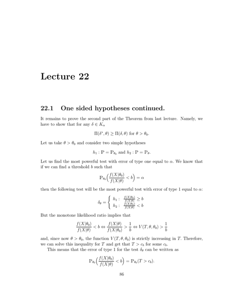
Lecture 22
22.1
One sided hypotheses continued.
It remains to prove the second part of the Theorem from last lecture. Namely, we
have to show that for any δ ∈ Kα
Π(δ ∗ , θ) ≥ Π(δ, θ) for θ > θ0 .
Let us take θ > θ0 and consider two simple hypotheses
h1 :
=
θ0
and h2 :
=
θ.
Let us find the most powerful test with error of type one equal to α. We know that
if we can find a threshold b such that
f (X|θ )
0
<b =α
θ0
f (X|θ)
then the following test will be the most powerful test with error of type 1 equal to α:
(
0)
h1 : ff(X|θ
≥b
(X|θ)
δθ =
f (X|θ0 )
h2 : f (X|θ) < b
But the monotone likelihood ratio implies that
f (X|θ0 )
f (X|θ)
1
1
<b⇔
> ⇔ V (T, θ, θ0 ) >
f (X|θ)
f (X|θ0 )
b
b
and, since now θ > θ0 , the function V (T, θ, θ0 ) is strictly increasing in T. Therefore,
we can solve this inequality for T and get that T > cb for some cb .
This means that the error of type 1 for the test δθ can be written as
f (X|θ )
0
< b = θ0 (T > cb ).
θ0
f (X|θ)
86
87
LECTURE 22.
But we chose this error to be equal to α = θ0 (T > c) which means that cb should
be such that
θ0 (T > cb ) =
θ0 (T > c) ⇒ c = cb .
Therefore,we proved that the test
δθ =
h1 : T ≤ c
h2 : T > c
is the most powerful test with error of type 1 equal to α.
But this test δθ is exactly the same as δ ∗ and it does not depend on θ. This means
that deciding between two simple hypotheses θ0 vs. θ one should always use the same
most powerful decision rule δ ∗ . But this means that δ ∗ is uniformly most powerful test
- what we wanted to prove. Notice that MLR played a key role here because thanks
to MLR the decision rule δθ was independent of θ. If δθ was different for different θ
this would mean that there is no UMP for composite hypotheses because it would be
advantageous to use different decision rules for different θ.
Example. Let us consider a family of normal distributions N (µ, 1) with unknown
mean µ as a parameter. Given some µ0 consider one sided hypotheses
H1 : µ ≤ µ0 and H2 : µ > µ0 .
As we have shown
Pn before the normal family N (µ, 1) has monotone likelihood ratio
with T (X) =
i=1 Xi . Therefore, the uniformly most powerful test with level of
significance α will be as follows:
P
H1 : Pni=1 Xi ≤ c
∗
δ =
n
H2 :
i=1 Xi > c.
The threshold c is determined by
α=
µ0 (T > c) =
µ0 (
X
Xi > c).
If the sample comes from N (µ0 , 1) then T has distribution N (nµ0 , n) and
n
1 X
Y =√
(Xi − µ0 ) ∼ N (0, 1)
n i=1
is standard normal. Therefore,
α=
µ0 (
n
X
i=1
Xi > c) =
µ0
n
c − nµ0 1 X
(Xi − µ0 ) > √
.
Y =√
n i=1
n
88
LECTURE 22.
Therefore, if using the table of standard normal distribution we find cα such that
(Y > cα ) = α then
√
c − nµ0
√
= cα or c = µ0 n + ncα .
n
Example. Let us now consider a family of normal distributions N (0, σ 2 ) with
variance σ 2 as unknown parameter. Given σ02 we consider one sided hypotheses
H1 : σ 2 ≤ σ02 and H2 : σ 2 > σ02 .
Let us first check if MLR holds in this case. The likelihood ratio is
Pn
Pn
2.
2
− 12
− 12
1
f (X|σ22 )
1
i=1 Xi
i=1 Xi
2σ2
2σ1
√
√
=
e
e
f (X|σ12 )
( 2πσ2 )n
( 2πσ1 )n
P 2
σ n
σ n
1
1
1
1
T
−
−
X
2
2
2
2
i
1
1
e 2σ1 2σ2
e 2σ1 2σ2 ,
=
=
σ2
σ2
Pn
2
2
2
where T =
i=1 Xi . When σ2 > σ1 the likelihood ratio is increasing in T and,
therefore, MLR holds. By the above Theorem, the UMP test exists and is given by
P
H1 : T = Pni=1 Xi2 ≤ c
∗
δ =
H2 : T = ni=1 Xi2 > c
where the threshold c is determined by
α=
σ02
(
n
X
Xi2
> c) =
i=1
σ02
n X
X 2
i
i=1
σ0
>
c
.
σ02
When Xi ∼ N (o, σ02 ), Xi /σ0 ∼ N (0, 1) are standard normal and, therefore,
n X
Xi 2
i=1
σ0
∼ χ2n
has χ2n distribution with n degrees of freedom. If we find cα such that χ2n (cα , ∞) = α
then c = cα σ02 .