March 11, 2004
18.413: Error-Correcting Codes Lab
Lecture 11
Lecturer: Daniel A. Spielman
11.1
Related Reading
• Fan, Chapter 2, Sections 3 and 4.
11.2
Belief Propagation on Trees
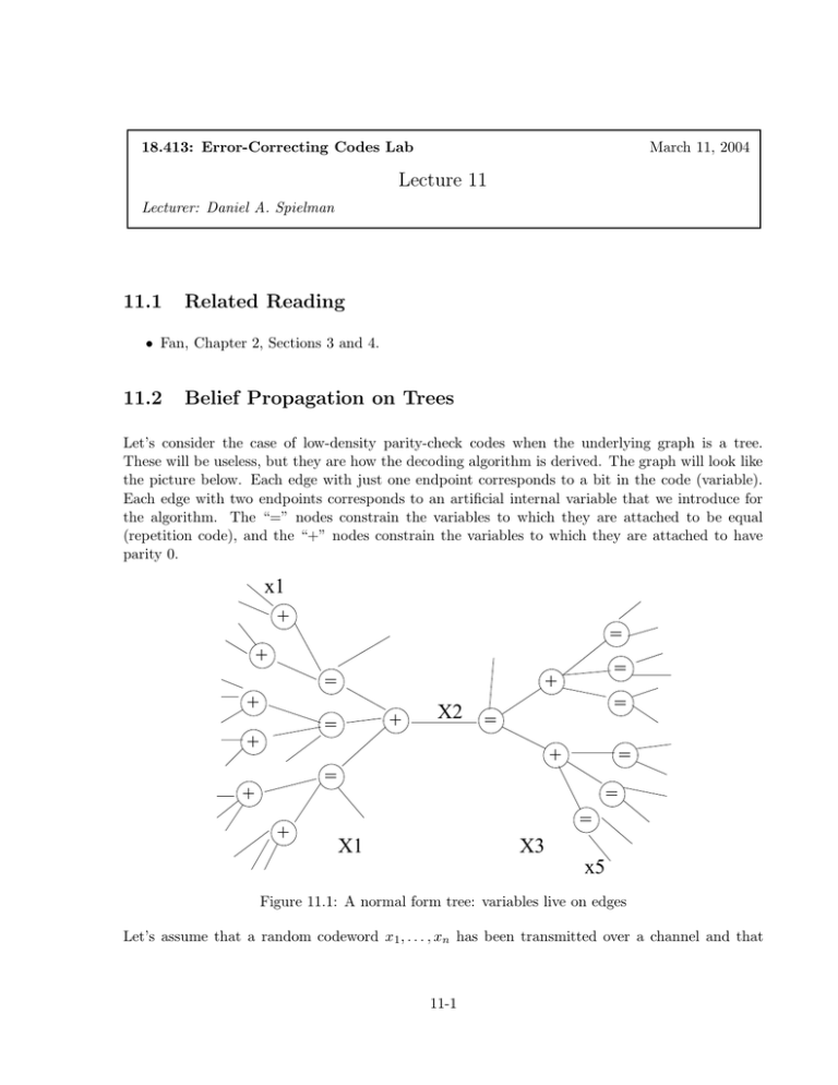
Let’s consider the case of low-density parity-check codes when the underlying graph is a tree.
These will be useless, but they are how the decoding algorithm is derived. The graph will look like
the picture below. Each edge with just one endpoint corresponds to a bit in the code (variable).
Each edge with two endpoints corresponds to an artificial internal variable that we introduce for
the algorithm. The “=” nodes constrain the variables to which they are attached to be equal
(repetition code), and the “+” nodes constrain the variables to which they are attached to have
parity 0.
x1
+
=
+
=
+
+
=
+
=
+
X2
=
=
=
+
=
+
+
=
=
X1
X3
x5
Figure 11.1: A normal form tree: variables live on edges
Let’s assume that a random codeword x 1 , . . . , xn has been transmitted over a channel and that
11-1
11-2
Lecture 11: March 11, 2004
b1 , . . . , bn has been received. We want to compute
Ppost [x1 = 0|b1 , . . . , bn ]
� Pext [x1 = 0|b1 ] Pext [x1 = 0|b2 , . . . , bn ] . (11.1)
So, we will focus on the computation of P ext [x1 = 0|b2 , . . . , bn ]. In particular, let’s look at what
information we need to pass over the edge whose variable in this figure is labeled X 2 . To do this,
we will group all the variables to the left of X 2 into one big clump, which we call X1 , and those to
the right into X3 .
By the three-variable lemma from lecture 6, we have
Lemma 11.2.1.
Pext [X1 = a1 |Y2 Y3 = b2 b3 ] =
�
P [X2 = a2 |X1 = a1 ] Pext [X2 = a2 |Y2 = b2 ] Pext [X2 = a2 |Y3 = b3 ] .
a2 :(a1 ,a2 )�C
.
As X2 is an internal variable, nothing is received from the channel for it, so there is no Y 2 or b2 .
So, the formula simplifies to
�
Pext [X1 = a1 |Y2 Y3 = b2 b3 ] =
P [X2 = a2 |X1 = a1 ] Pext [X2 = a2 |Y3 = b3 ] .
a2 :(a1 ,a2 )�C
. Thus, the only information about X3 that needs to be passed through variable X 2 is
Pext [X2 = a2 |Y3 = b3 ] .
Also, since X2 is a just one bit, we only need this information for a 2 � {0, 1}.
Now, I told you that we were interested in x 1 , not X1 . But, if we can compute probability estimates
for X1 , then we can do the same for x1 . So, the same information is what is required.
This begs the question of how we compute P ext [X2 = a2 |Y3 = b3 ] . The answer is that we look
back one step in the tree, and consider the other edges entering the “=” node to the right of X 2 .
Each of these can pass up a similar message about the subtree beneath them. Then, the “=”
node combines all of these estimates according to the rule for the repetition code. Of course, these
message came through “+” nodes, which combine their incomming messages according to the rule
for parity codes.
11.3
Dynamic programming
This description of computing Ppost [x1 = 0|b2 , . . . , bn ] has one defect: it is doing a whole lot of
work just for x1 , and if we want to do it again for some other variable, such as x 5 , we would have
to do it all over again. However, if you take a look at the algorithm, most of the computations are
the same of both variables. In fact, it is possible to perform all the computations for all variables
at once while doing little more work that one does for just one variable. The idea is to use the
following rule:
Lecture 11: March 11, 2004
11-3
The message a node sends out along an edge should be the corresponding function
of the messages that come in on every other edge.
There is a natural was of describing the resulting algorithm in an object-oriented fashion. In this
case, each node will correspond to an object. Each node will store all of its incomming messages.
As soon as it has an incomming message on all but one of its edges, it sends a message to the node
on the other end of the remaining edge. When it has messages on every incomming edge, it sends
messages to the nodes at the end of all the other edges. To get this process started, we note that
the the channel outputs correspond to a message on each external edge (with one endpoint), so each
node that has just one internal edge will be ready as soon as the channel outputs are processed.
Also note that, at the end of the algorithm, a message will be sent to each external edge. This will
contain the desired extrinsic probability estimation.
The algorithm described above is rather asynchronos: I’ve described a sufficient algorithm in terms
of passing messages, and it works regardless of the order in which messages are delivered (as long
as they all get delivered). A tighter algorithm would have a top-down flow control: we would
pick some central node to call the “root”. Then, nodes would fire in an order depending on their
distance to the root. First, every node that is furthest from the root would fire one message. Then,
those in the next level would fire one message, etc. This would repeat until we got to the root. The
root would have all of its incomming messages, and so could send out all of its outgoing messsges.
This would then be true of the nodes a distance 1 from the root, etc. So, the messages would then
propogate back down the tree.
11.4
Infinite trees
What if the tree were infinite? In that case, there would be no nodes of maximum distance from
the root. We can make a version of this algorithm work anyway. The idea is to proceed in rounds,
and begin by putting a null message incomming on each edge on the first round. That way, each
“=” node will have a null message on every edge in the first round, where a null message means half
probability zero and half probability one. That way, each “=” node will send an outgoing message
on each of its edges. In the next round, this will mean that each “+” node has an incomming
message, and so will send an outgoing message. Then, each “=” has an incomming message, etc.
If we let this go for k rounds, then the messages being sent out on the external edges will look like
the messages we would have created using the tree algorithm on the tree of depth k surrounding
that edge.
11.5
Small Project 2
You should verify for yourself that this tree algorithm is exactly what we implemented in small
project 2, and that you could have sped it up by using the dymanic programming idea.
During class yesterday, Boris observed that the naive decoding algorithm didn’t do all that much
better than just rounding the bits, at least for large �. So that you can see this, here are three
11-4
Lecture 11: March 11, 2004
plots: one for the bit error probability of just rounding the received signal (dotted line with circles),
one for the class N0 (solid line with circles), and a theoretical curve I will explain in a moment
(dashed line with squares).
0.35
0.3
0.25
BER
0.2
N0
rounding
theory
0.15
0.1
0.05
0
0.4
0.6
2
1.8
1.6
1.4
1.2
sigma
1
0.8
It becomes clearer that the coding really is achieving something if you look at the log-log chart:
0
10
−1
BER
10
−2
10
N0
rounding
theory
−3
10
−4
10
−0.3
10
−0.2
10
−0.1
0
10
10
0.1
10
0.2
10
0.3
10
sigma
In particular, the two curves have different slopes.
The theoretical curve is an attempt to explain the performance of the naive algorithm, up to the
first order. To do this, let p denote the probability of an error after rounding. If there is only one
error, it will probably be corrected. If some bit is in error, and there is another error, let’s just
assume that the algorithm cannot correct the first bit. (although this is a little pessimistic). Thus,
11-5
Lecture 11: March 11, 2004
we estimate the probability of a bit error to be
p(1 − (1 − p)8 ).
This is what I’ve plotted in the theoretical curve. At first, this curve should not be too different
from the rounding curve, because (1 − p) 8 will be quite small, so it will be likely that there is
another error. On the other hand, for p small, this error probability is approximately 8p 2 . Thus,
it grows much smaller than p for small p, which explains why the slope of the error curve in the
log-log chart for the N0 line should be twice the slope for the rounding line.