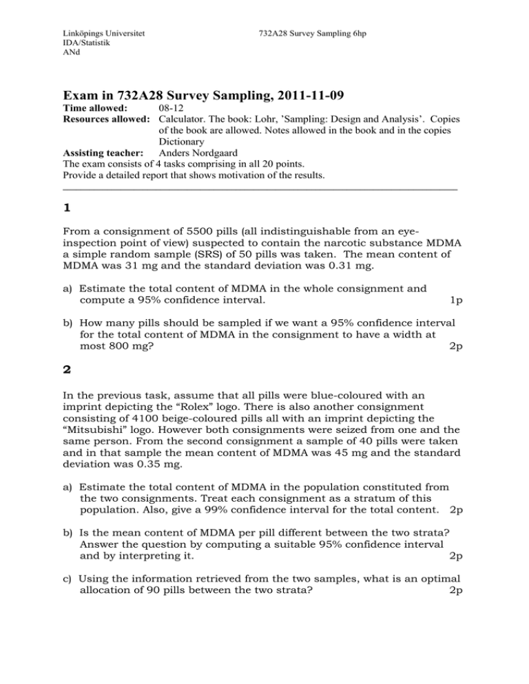
Linköpings Universitet
IDA/Statistik
ANd
732A28 Survey Sampling 6hp
Exam in 732A28 Survey Sampling, 2011-11-09
Time allowed:
08-12
Resources allowed: Calculator. The book: Lohr, ’Sampling: Design and Analysis’. Copies
of the book are allowed. Notes allowed in the book and in the copies
Dictionary
Assisting teacher: Anders Nordgaard
The exam consists of 4 tasks comprising in all 20 points.
Provide a detailed report that shows motivation of the results.
_________________________________________________________________________________________
1
From a consignment of 5500 pills (all indistinguishable from an eyeinspection point of view) suspected to contain the narcotic substance MDMA
a simple random sample (SRS) of 50 pills was taken. The mean content of
MDMA was 31 mg and the standard deviation was 0.31 mg.
a) Estimate the total content of MDMA in the whole consignment and
compute a 95% confidence interval.
1p
b) How many pills should be sampled if we want a 95% confidence interval
for the total content of MDMA in the consignment to have a width at
most 800 mg?
2p
2
In the previous task, assume that all pills were blue-coloured with an
imprint depicting the “Rolex” logo. There is also another consignment
consisting of 4100 beige-coloured pills all with an imprint depicting the
“Mitsubishi” logo. However both consignments were seized from one and the
same person. From the second consignment a sample of 40 pills were taken
and in that sample the mean content of MDMA was 45 mg and the standard
deviation was 0.35 mg.
a) Estimate the total content of MDMA in the population constituted from
the two consignments. Treat each consignment as a stratum of this
population. Also, give a 99% confidence interval for the total content. 2p
b) Is the mean content of MDMA per pill different between the two strata?
Answer the question by computing a suitable 95% confidence interval
and by interpreting it.
2p
c) Using the information retrieved from the two samples, what is an optimal
allocation of 90 pills between the two strata?
2p
3
Let us assume we would like to poll the opinions about the current “Eurocrisis” in a middle-sized town of Sweden. To simplify this survey we divide
the town into 50 living areas, where each area can be assumed to consist of
a mixture of individuals with respect to their opinions about the subject.
The survey is made by drawing a SRS of 4 living areas and in each area
interviewing a SRS of 50 individuals (older than 15 years). Each individual in
the sample is asked a number of questions of which one is “Do you think the
European Monetary Union (EMU) will exist in ten years time?” Valid answers
to that question are “yes”, “no” or “don’t know”.
The number of individuals above 15 in the town is approximately 32150.
The results are summarised as
Area Approx. number individuals (above 15) Number of “yes”
living in area
1
550
33
2
610
38
3
740
31
4
480
33
Note that the sample of living areas is unusually small in this example, but
use normality assumptions in spite of this.
a) Compute a ratio estimate of the proportion individuals (above 15) that
would answer yes to the question (i.e., thinks EMU will exist in ten years
time). Also compute a 99% confidence interval for this proportion.
2p
b) Without making any calculations, motivate in this case which of a ratio
estimate and unbiased estimate would be the most efficient.
1p
c) Is the sample made self-weighing? Motivate shortly.
1p
d) Assume now that the sampling of living areas was made with replacement
and with probabilities proportional to the approximate number of
individuals (above 15) living in them . Compute a new point estimate of
the proportion of individuals (above 15) that would answer yes to the
question and a 95% confidence interval for this proportion.
2p
4
A questionnaire was sent to a SRS of 200 individuals belonging to a
population of 10000. Among the questions were “How much money did you
save in funds of different kinds in the year 2010?” and “How large was your
annual salary for 2010?”. Of main interest is the first question, while the
second question is there more to classify the respondents.
The response rate was not that impressive, 45%, but the survey conductors
still carried on with the responses they got. For the respondents of the
survey the total amount that had been saved in funds 2010 was 1 085 000
SEK and the standard deviation of the answers was 5160 SEK. The
summarised annual salaries for the respondents were 28 080 000 SEK and
the standard deviation was 38 300 SEK. In the whole population the mean
annual salary is 313 100 SEK. Moreover, the correlation between answered
amount of saving and annual salary was found to be approximately 0.77.
a) Estimate the total amount of savings in funds 2010 in the population by
using a ratio estimate were annual salary is the auxiliary variable. Also
compute a 95% confidence interval. (Hint: Express the data in thousands
of SEK to make calculations easier)
2p
b) In the population about 75% of the individuals have annual salaries
below 330 000 SEK. In the sample the mean amount of savings in funds
for 2010 for individuals belonging to this group was 9300 SEK and for
the rest of the individuals in the sample the corresponding mean was
19100. Compute a post-stratified estimate of the total amount of savings
in funds 2010 for the whole population.
1p
c) In tasks a) and b) what assumptions have been made about the nonresponse for the estimates to be valid?
1p
d) It is not unrealistic to believe that we may have access to the annual
salaries of all individuals of the original sample, i.e. for both respondents
and non-respondents. How could this help us to handle the nonresponse? What assumptions are needed for this?
1p
Area between 0 and z
0.00
0.01
0.02
0.03
0.04
0.05
0.06
0.07
0.08
0.09
0.0 0.0000 0.0040 0.0080 0.0120 0.0160 0.0199 0.0239 0.0279 0.0319 0.0359
0.1 0.0398 0.0438 0.0478 0.0517 0.0557 0.0596 0.0636 0.0675 0.0714 0.0753
0.2 0.0793 0.0832 0.0871 0.0910 0.0948 0.0987 0.1026 0.1064 0.1103 0.1141
0.3 0.1179 0.1217 0.1255 0.1293 0.1331 0.1368 0.1406 0.1443 0.1480 0.1517
0.4 0.1554 0.1591 0.1628 0.1664 0.1700 0.1736 0.1772 0.1808 0.1844 0.1879
0.5 0.1915 0.1950 0.1985 0.2019 0.2054 0.2088 0.2123 0.2157 0.2190 0.2224
0.6 0.2257 0.2291 0.2324 0.2357 0.2389 0.2422 0.2454 0.2486 0.2517 0.2549
0.7 0.2580 0.2611 0.2642 0.2673 0.2704 0.2734 0.2764 0.2794 0.2823 0.2852
0.8 0.2881 0.2910 0.2939 0.2967 0.2995 0.3023 0.3051 0.3078 0.3106 0.3133
0.9 0.3159 0.3186 0.3212 0.3238 0.3264 0.3289 0.3315 0.3340 0.3365 0.3389
1.0 0.3413 0.3438 0.3461 0.3485 0.3508 0.3531 0.3554 0.3577 0.3599 0.3621
1.1 0.3643 0.3665 0.3686 0.3708 0.3729 0.3749 0.3770 0.3790 0.3810 0.3830
1.2 0.3849 0.3869 0.3888 0.3907 0.3925 0.3944 0.3962 0.3980 0.3997 0.4015
1.3 0.4032 0.4049 0.4066 0.4082 0.4099 0.4115 0.4131 0.4147 0.4162 0.4177
1.4 0.4192 0.4207 0.4222 0.4236 0.4251 0.4265 0.4279 0.4292 0.4306 0.4319
1.5 0.4332 0.4345 0.4357 0.4370 0.4382 0.4394 0.4406 0.4418 0.4429 0.4441
1.6 0.4452 0.4463 0.4474 0.4484 0.4495 0.4505 0.4515 0.4525 0.4535 0.4545
1.7 0.4554 0.4564 0.4573 0.4582 0.4591 0.4599 0.4608 0.4616 0.4625 0.4633
1.8 0.4641 0.4649 0.4656 0.4664 0.4671 0.4678 0.4686 0.4693 0.4699 0.4706
1.9 0.4713 0.4719 0.4726 0.4732 0.4738 0.4744 0.4750 0.4756 0.4761 0.4767
2.0 0.4772 0.4778 0.4783 0.4788 0.4793 0.4798 0.4803 0.4808 0.4812 0.4817
2.1 0.4821 0.4826 0.4830 0.4834 0.4838 0.4842 0.4846 0.4850 0.4854 0.4857
2.2 0.4861 0.4864 0.4868 0.4871 0.4875 0.4878 0.4881 0.4884 0.4887 0.4890
2.3 0.4893 0.4896 0.4898 0.4901 0.4904 0.4906 0.4909 0.4911 0.4913 0.4916
2.4 0.4918 0.4920 0.4922 0.4925 0.4927 0.4929 0.4931 0.4932 0.4934 0.4936
2.5 0.4938 0.4940 0.4941 0.4943 0.4945 0.4946 0.4948 0.4949 0.4951 0.4952
2.6 0.4953 0.4955 0.4956 0.4957 0.4959 0.4960 0.4961 0.4962 0.4963 0.4964
2.7 0.4965 0.4966 0.4967 0.4968 0.4969 0.4970 0.4971 0.4972 0.4973 0.4974
2.8 0.4974 0.4975 0.4976 0.4977 0.4977 0.4978 0.4979 0.4979 0.4980 0.4981
2.9 0.4981 0.4982 0.4982 0.4983 0.4984 0.4984 0.4985 0.4985 0.4986 0.4986
3.0 0.4987 0.4987 0.4987 0.4988 0.4988 0.4989 0.4989 0.4989 0.4990 0.4990